# Install the necessary dependencies

import os
import sys
!{sys.executable} -m pip install --quiet pandas scikit-learn numpy matplotlib jupyterlab_myst ipython

12.2. More classifiers

In this section, you will use the dataset you saved from the last section full of balanced, clean data all about cuisines.

You will use this dataset with a variety of classifiers to predict a given national cuisine based on a group of ingredients. While doing so, you’ll learn more about some of the ways that algorithms can be leveraged for classification tasks.

12.2.1. Exercise - predict a national cuisine

1. Working in this section’s build-classification-models file, import that file along with the Pandas library:

import pandas as pd
cuisines_df = pd.read_csv("https://static-1300131294.cos.ap-shanghai.myqcloud.com/data/classification/cleaned_cuisines.csv")
cuisines_df.head()

	Unnamed: 0	cuisine	almond	angelica	anise	anise_seed	apple	apple_brandy	apricot	armagnac	...	whiskey	white_bread	white_wine	whole_grain_wheat_flour	wine	wood	yam	yeast	yogurt	zucchini
0	0	indian	0	0	0	0	0	0	0	0	...	0	0	0	0	0	0	0	0	0	0
1	1	indian	1	0	0	0	0	0	0	0	...	0	0	0	0	0	0	0	0	0	0
2	2	indian	0	0	0	0	0	0	0	0	...	0	0	0	0	0	0	0	0	0	0
3	3	indian	0	0	0	0	0	0	0	0	...	0	0	0	0	0	0	0	0	0	0
4	4	indian	0	0	0	0	0	0	0	0	...	0	0	0	0	0	0	0	0	1	0

5 rows × 382 columns

2. Now, import several more libraries:

from sklearn.linear_model import LogisticRegression
from sklearn.model_selection import train_test_split, cross_val_score
from sklearn.metrics import accuracy_score,precision_score,confusion_matrix,classification_report, precision_recall_curve
from sklearn.svm import SVC
import numpy as np

3. Divide the x and y coordinates into two dataframes for training. cuisine can be the labels dataframe:

cuisines_label_df = cuisines_df['cuisine']
cuisines_label_df.head()

0    indian
1    indian
2    indian
3    indian
4    indian
Name: cuisine, dtype: object

4. Drop that Unnamed: 0 column and the cuisine column, calling drop(). Save the rest of the data as trainable features:

cuisines_feature_df = cuisines_df.drop(['Unnamed: 0', 'cuisine'], axis=1)
cuisines_feature_df.head()

	almond	angelica	anise	anise_seed	apple	apple_brandy	apricot	armagnac	artemisia	artichoke	...	whiskey	white_bread	white_wine	whole_grain_wheat_flour	wine	wood	yam	yeast	yogurt	zucchini
0	0	0	0	0	0	0	0	0	0	0	...	0	0	0	0	0	0	0	0	0	0
1	1	0	0	0	0	0	0	0	0	0	...	0	0	0	0	0	0	0	0	0	0
2	0	0	0	0	0	0	0	0	0	0	...	0	0	0	0	0	0	0	0	0	0
3	0	0	0	0	0	0	0	0	0	0	...	0	0	0	0	0	0	0	0	0	0
4	0	0	0	0	0	0	0	0	0	0	...	0	0	0	0	0	0	0	0	1	0

5 rows × 380 columns

Now you are ready to train your model!

12.2.2. Choosing your classifier

Now that your data is clean and ready for training, you have to decide which algorithm to use for the job.

Scikit-learn groups classification under Supervised Learning, and in that category you will find many ways to classify. The variety is quite bewildering at first sight. The following methods all include classification techniques:

• Linear Models

• Support Vector Machines

• Stochastic Gradient Descent

• Nearest Neighbors

• Gaussian Processes

• Decision Trees

• Ensemble methods (voting Classifier)

• Multiclass and multioutput algorithms (multiclass and multilabel classification, multiclass-multioutput classification)

See also

You can also use neural networks to classify data, but that is outside the scope of this section.

12.2.2.1. What classifier to go with?

So, which classifier should you choose? Often, running through several and looking for a good result is a way to test. Scikit-learn offers a side-by-side comparison on a created dataset, comparing KNeighbors, SVC two ways, GaussianProcessClassifier, DecisionTreeClassifier, RandomForestClassifier, MLPClassifier, AdaBoostClassifier, GaussianNB and QuadraticDiscrinationAnalysis, showing the results visualized:

Fig. 12.3 Comparison of classifiers 🔗source

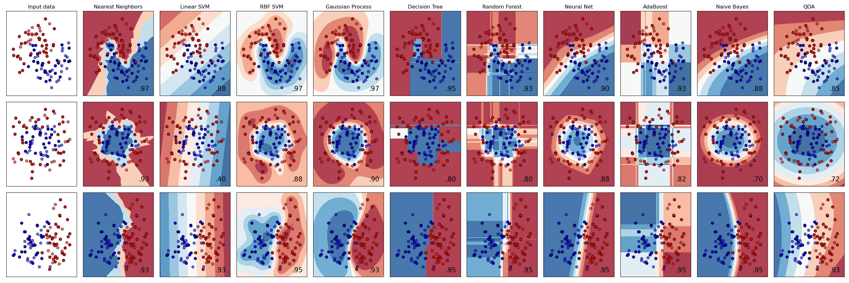
See also

Plots generated on Scikit-learn’s documentation.

AutoML solves this problem neatly by running these comparisons in the cloud, allowing you to choose the best algorithm for your data. Try it here.

12.2.2.2. A better approach

A better way than wildly guessing, however, is to follow the ideas on this downloadable ML Cheat sheet. Here, we discover that, for our multiclass problem, we have some choices:

Fig. 12.4 Cheatsheet for multiclass problems 🔗source

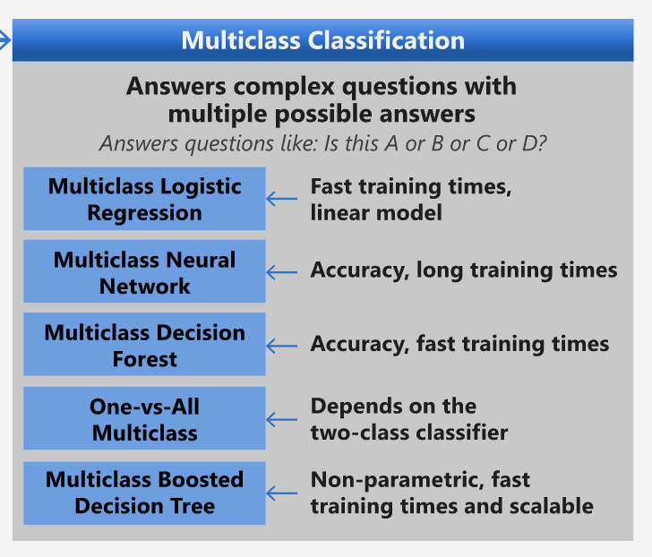
Note

A section of Microsoft’s Algorithm Cheat Sheet, detailing multiclass classification options.

See also

Download this cheat sheet, print it out, and hang it on your wall!

12.2.2.3. Reasoning

Let’s see if we can reason our way through different approaches given the constraints we have:

• Neural networks are too heavy. Given our clean, but minimal dataset, and the fact that we are running training locally via notebooks, neural networks are too heavyweight for this task.

• No two-class classifier. We do not use a two-class classifier, so that rules out one-vs-all.

• Decision tree or logistic regression could work. A decision tree might work, or logistic regression for multiclass data.

• Multiclass Boosted Decision Trees solve a different problem. The multiclass boosted decision tree is most suitable for nonparametric tasks, e.g. tasks designed to build rankings, so it is not useful for us.

12.2.2.4. Using Scikit-learn

We will be using Scikit-learn to analyze our data. However, there are many ways to use logistic regression in Scikit-learn. Take a look at the parameters to pass.

Essentially there are two important parameters - multi_class and solver - that we need to specify, when we ask Scikit-learn to perform a logistic regression. The multi_class value applies a certain behavior. The value of the solver is what algorithm to use. Not all solvers can be paired with all multi_class values.

According to the docs, in the multiclass case, the training algorithm:

• Uses the one-vs-rest (OvR) scheme, if the multi_class option is set to ovr.

• Uses the cross-entropy loss, if the multi_class option is set to multinomial. (Currently the multinomial option is supported only by the ‘lbfgs’, ‘sag’, ‘saga’ and ‘newton-cg’ solvers.)

See also

The ‘scheme’ here can either be ‘ovr’ (one-vs-rest) or ‘multinomial’. Since logistic regression is really designed to support binary classification, these schemes allow it to better handle multiclass classification tasks. 🔗source

The ‘solver’ is defined as “the algorithm to use in the optimization problem”. source.

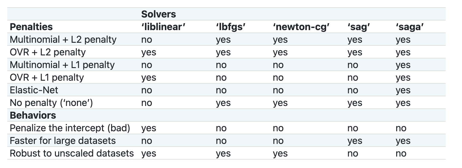
Scikit-learn offers this table to explain how solvers handle different challenges presented by different kinds of data structures:

Fig. 12.5 Solvers 🔗source

12.2.3. Exercise - split the data

We can focus on logistic regression for our first training trial since you recently learned about the latter in a previous section. Split your data into training and testing groups by calling train_test_split():

X_train, X_test, y_train, y_test = train_test_split(cuisines_feature_df, cuisines_label_df, test_size=0.3)

12.2.4. Exercise - apply logistic regression

Since you are using the multiclass case, you need to choose what scheme to use and what solver to set. Use LogisticRegression with a multiclass setting and the liblinear solver to train.

1. Create a logistic regression with multi_class set to ovr and the solver set to liblinear:

lr = LogisticRegression(multi_class='ovr',solver='liblinear')
model = lr.fit(X_train, np.ravel(y_train))

accuracy = model.score(X_test, y_test)
print ("Accuracy is {}".format(accuracy))

Accuracy is 0.79232693911593

See also

Try a different solver like lbfgs, which is often set as default.

Note

Use Pandas ravel function to flatten your data when needed.

The accuracy is good at over 80%!

2. You can see this model in action by testing one row of data (#50):

print(f'ingredients: {X_test.iloc[50][X_test.iloc[50]!=0].keys()}')
print(f'cuisine: {y_test.iloc[50]}')

ingredients: Index(['cayenne', 'cilantro', 'cumin', 'lime', 'pineapple', 'tomato',
       'vegetable_oil'],
      dtype='object')
cuisine: indian

See also

Try a different row number and check the results.

3. Digging deeper, you can check for the accuracy of this prediction:

test= X_test.iloc[50].values.reshape(-1, 1).T
proba = model.predict_proba(test)
classes = model.classes_
resultdf = pd.DataFrame(data=proba, columns=classes)

topPrediction = resultdf.T.sort_values(by=[0], ascending = [False])
topPrediction.head()

/usr/share/miniconda/envs/open-machine-learning-jupyter-book/lib/python3.9/site-packages/sklearn/base.py:409: UserWarning: X does not have valid feature names, but LogisticRegression was fitted with feature names
  warnings.warn(

	0
indian	0.866546
thai	0.123433
chinese	0.008208
korean	0.000927
japanese	0.000886

See also

Can you explain why the model is pretty sure this is an Indian cuisine?

4. Get more detail by printing a classification report, as you did in the regression sections:

y_pred = model.predict(X_test)
print(classification_report(y_test,y_pred))

              precision    recall  f1-score   support

     chinese       0.72      0.72      0.72       230
      indian       0.92      0.87      0.90       249
    japanese       0.76      0.76      0.76       249
      korean       0.84      0.71      0.77       238
        thai       0.74      0.91      0.81       233

    accuracy                           0.79      1199
   macro avg       0.80      0.79      0.79      1199
weighted avg       0.80      0.79      0.79      1199

12.2.5. Your turn! 🚀

In this section, you used your cleaned data to build a machine learning model that can predict a national cuisine based on a series of ingredients. Take some time to read through the many options Scikit-learn provides to classify data. Dig deeper into the concept of ‘solver’ to understand what goes on behind the scenes.

Assignment - Study the solvers.

12.2.6. Acknowledgments

Thanks to Microsoft for creating the open-source course ML-For-Beginners. It inspires the majority of the content in this chapter.