Linear Regression Metrics
Contents
42.46. Linear Regression Metrics#
Linear regression is a fundamental and widely used technique in machine learning and statistics for predicting continuous values based on input variables. It finds its application in various domains, from finance and economics to healthcare and engineering. When using linear regression, it’s essential to assess the model’s performance accurately. This is where linear regression metrics come into play.
In this tutorial, we will delve into the world of linear regression metrics, exploring the key evaluation measures that allow us to gauge how well a linear regression model fits the data and makes predictions. These metrics provide valuable insights into the model’s accuracy, precision, and ability to capture the underlying relationships between variables.
We will cover essential concepts such as Mean Squared Error (MSE), Root Mean Squared Error (RMSE), R-squared (R2) score, and Mean Absolute Error (MAE). Understanding these metrics is crucial for data scientists, machine learning practitioners, and anyone looking to harness the power of linear regression for predictive modeling.
Whether you are building models for price predictions, sales forecasts, or any other regression task, mastering these metrics will empower you to make informed decisions and fine-tune your models for optimal performance. Let’s embark on this journey to explore the intricacies of linear regression metrics and enhance our ability to assess and improve regression models.
42.46.1. Mean Squared Error (MSE)#
In the realm of linear regression metrics, one fundamental measure of model performance is the Mean Squared Error (MSE). MSE serves as a valuable indicator of how well your linear regression model aligns its predictions with the actual data points. This metric quantifies the average of the squared differences between predicted values and observed values.
42.46.1.1. The Formula#
Mathematically, the MSE is computed using the following formula:
Where:
\(n\) is the number of data points.
\(y_i\) represents the actual observed value for the \(i^{th}\) data point.
\(\hat{y}_i\) represents the predicted value for the \(i^{th}\) data point.
42.46.1.2. Interpretation#
A lower MSE value indicates that the model’s predictions are closer to the actual values, signifying better model performance. Conversely, a higher MSE suggests that the model’s predictions deviate more from the true values, indicating poorer performance.
42.46.1.3. Python Implementation#
Let’s take a look at how to calculate MSE in Python. We’ll use a simple example with sample data:
# Import necessary libraries
import numpy as np

# Sample data for demonstration (replace with your actual data)
actual_values = np.array([22.1, 19.9, 24.5, 20.1, 18.7])
predicted_values = np.array([23.5, 20.2, 23.9, 19.8, 18.5])

# Calculate the squared differences between actual and predicted values
squared_errors = (actual_values - predicted_values) ** 2

# Calculate the mean of squared errors to get MSE
mse = np.mean(squared_errors)

# Print the MSE
print("Mean Squared Error (MSE):", mse)
Mean Squared Error (MSE): 0.5079999999999996
42.46.2. Root Mean Squared Error (RMSE)#
The Root Mean Squared Error (RMSE) is another important metric for evaluating the performance of a linear regression model. It is the square root of the Mean Squared Error (MSE) and provides a measure of the average magnitude of error between actual and predicted values.
42.46.2.1. The Formula#
The formula for RMSE is:
Where:
\(n\) is the number of data points
\(y_i \) represents the actual value of the dependent variable
\( \hat{y}_i \) represents the predicted value of the dependent variable
42.46.2.2. Python Implementation#
# Calculate RMSE
rmse = np.sqrt(mse)

# Print the RMSE
print("Root Mean Squared Error (RMSE):", rmse)
Root Mean Squared Error (RMSE): 0.7127411872482181
42.46.3. R-squared (R2) Score#
The R-squared (R2) score, also known as the coefficient of determination, is a measure that indicates the proportion of the variance in the dependent variable that is predictable from the independent variables. It provides insight into how well the model is performing compared to a simple mean.
42.46.3.1. The Formula#
The formula for R2 score is:
Where:
\( n \) is the number of data points
\( y_i \) represents the actual value of the dependent variable
\( \hat{y}_i \) represents the predicted value of the dependent variable
\( \bar{y} \) is the mean of the dependent variable
42.46.3.2. Python Implementation#
# Calculate the mean of actual values
mean_actual = np.mean(actual_values)

# Calculate the total sum of squares
total_sum_squares = np.sum((actual_values - mean_actual) ** 2)

# Calculate the residual sum of squares
residual_sum_squares = np.sum(squared_errors)

# Calculate R2 score
r2_score = 1 - (residual_sum_squares / total_sum_squares)

# Print the R2 score
print("R-squared (R2) Score:", r2_score)
R-squared (R2) Score: 0.8776021588280649
42.46.4. Residual Analysis#
Residual analysis is a critical step in evaluating the performance of a linear regression model. It involves examining the differences between the observed and predicted values (i.e., the residuals). This helps us understand if there are any patterns or trends that the model might have missed.
42.46.4.1. Python Implementation#
import matplotlib.pyplot as plt
'''
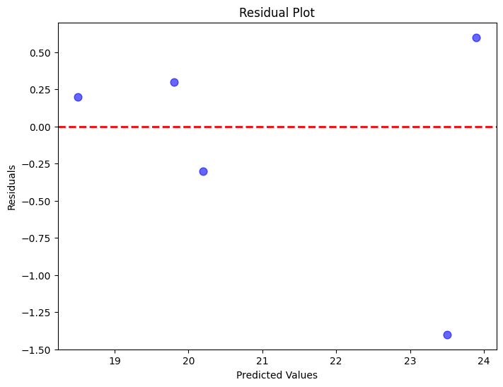
In this code, we first calculate the residuals by subtracting the predicted values from the actual values. Then, we create a scatter plot of predicted values against residuals. The red dashed line at y=0 is a reference line; ideally, we want the residuals to be evenly distributed around this line.
'''
# Calculate residuals
residuals = actual_values - predicted_values
# Plotting residuals
plt.figure(figsize=(8, 6))
plt.scatter(predicted_values, residuals, c='b', s=60, alpha=0.6)
plt.axhline(y=0, color='r', linestyle='--', linewidth=2)
plt.title("Residual Plot")
plt.xlabel("Predicted Values")
plt.ylabel("Residuals")
plt.show()
42.46.4.2. Interpretation#
If the residuals are randomly scattered around the red line, it suggests that the model is capturing the underlying patterns in the data well. If there’s a clear pattern in the residuals (e.g., a curve or a trend), it indicates that the model might be missing some important features. Residual analysis is a crucial step in understanding the limitations of the model and can provide insights into potential areas of improvement.
42.46.5. Mean Absolute Error (MAE)#
The Mean Absolute Error (MAE) is a metric that measures the average absolute differences between actual and predicted values. Unlike MSE, MAE does not square the differences, which makes it less sensitive to outliers.
42.46.5.1. The Formula#
The formula for Mean Absolute Errord is: $\( MAE = \frac{1}{n} \sum_{i=1}^{n} |y_i - \hat{y}_i| \)$ Where:
\( n \) is the number of data points
\( y_i \) represents the actual value of the dependent variable
\( \hat{y}_i \) represents the predicted value of the dependent variable
42.46.5.2. Python Implementation#
# Calculate absolute differences between actual and predicted values
absolute_errors = np.abs(actual_values - predicted_values)

# Calculate the mean of absolute errors to get MAE
mae = np.mean(absolute_errors)

# Print the MAE
print("Mean Absolute Error (MAE):", mae)
Mean Absolute Error (MAE): 0.5600000000000002
42.46.5.3. Interpretation#
The MAE gives us an average of how far off our predictions are from the actual values. It provides a more intuitive understanding of error compared to MSE.
42.46.6. Mean Absolute Percentage Error (MAPE)#
The Mean Absolute Percentage Error (MAPE) is a metric used to evaluate the accuracy of a model’s predictions in percentage terms. It measures the average absolute percentage difference between actual and predicted values.
42.46.6.1. The Formula#
The formula for MAPE is:
Where:
\( n \) is the number of data points
\( y_i \) represents the actual value of the dependent variable
\( \hat{y}_i \) represents the predicted value of the dependent variable
42.46.6.2. Interpretation#
# Calculate absolute percentage differences between actual and predicted values
absolute_percentage_errors = np.abs((actual_values - predicted_values) / actual_values) * 100

# Calculate the mean of absolute percentage errors to get MAPE
mape = np.mean(absolute_percentage_errors)

# Print the MAPE
print("Mean Absolute Percentage Error (MAPE):", mape)
Mean Absolute Percentage Error (MAPE): 2.5706829878497204
42.46.7. Conclusion and Recap#
In this tutorial, we covered several important metrics used to evaluate the performance of linear regression models. Here’s a quick recap:
Mean Squared Error (MSE): Measures the average squared difference between actual and predicted values.
Root Mean Squared Error (RMSE): The square root of MSE, providing a measure of the average magnitude of error.
R-squared (R2) Score: Indicates the proportion of the variance in the dependent variable that is predictable from the independent variables.
Mean Absolute Error (MAE): Measures the average absolute differences between actual and predicted values.
Mean Absolute Percentage Error (MAPE): Measures the average absolute percentage difference between actual and predicted values.
Each of these metrics provides unique insights into the performance of a linear regression model. Choosing the right metric depends on the specific characteristics of the data and the objectives of the modeling task.
By understanding and utilizing these metrics, you can make informed decisions about the accuracy and reliability of your linear regression models.