Case Study: Debugging in Regression
Contents
LICENSE
Copyright 2018 Google LLC.
Licensed under the Apache License, Version 2.0 (the “License”); you may not use this file except in compliance with the License. You may obtain a copy of the License at
https://www.apache.org/licenses/LICENSE-2.0
Unless required by applicable law or agreed to in writing, software distributed under the License is distributed on an “AS IS” BASIS, WITHOUT WARRANTIES OR CONDITIONS OF ANY KIND, either express or implied. See the License for the specific language governing permissions and limitations under the License.
42.88. Case Study: Debugging in Regression#
In this Colab, you will learn how to debug a regression problem through a case study. You will:
Set up the problem.
Interpret the correlation matrix.
Implement linear and nonlinear models.
Compare and choose between linear and nonlinear models.
Optimize your chosen model.
Debug your chosen model.
42.88.1. Setup#
This Colab uses the wine quality dataset<sup#[1]</sup#, which is hosted at UCI. This dataset contains data on the physicochemical properties of wine along with wine quality ratings. The problem is to predict wine quality (0-10) from physicochemical properties.
Please make a copy of this Colab before running it. Click on File, and then click on Save a copy in Drive.
<small#[1] Modeling wine preferences by data mining from physicochemical properties. P. Cortez, A. Cerdeira, F. Almeida, T. Matos and J. Reis. Decision Support Systems, Elsevier, 47(4):547-553, 2009.</small#
Load libraries and data by running the next cell. Display the first few rows to verify that the dataset loaded correctly.
# Reset environment for a new run
%reset -f

# Load libraries
from os.path import join # for joining file pathnames
import pandas as pd
import seaborn as sns
import tensorflow as tf
from tensorflow import keras
import numpy as np
import matplotlib.pyplot as plt

# Set Pandas display options
pd.options.display.max_rows = 10
pd.options.display.float_format = '{:.1f}'.format

wineDf = pd.read_csv(
  "https://static-1300131294.cos.ap-shanghai.myqcloud.com/data/winequality.csv",
  encoding='latin-1')
wineDf.columns = ['fixed acidity','volatile acidity','citric acid',
                     'residual sugar','chlorides','free sulfur dioxide',
                     'total sulfur dioxide','density','pH',
                     'sulphates','alcohol','quality']
wineDf.head()
| fixed acidity | volatile acidity | citric acid | residual sugar | chlorides | free sulfur dioxide | total sulfur dioxide | density | pH | sulphates | alcohol | quality | |
|---|---|---|---|---|---|---|---|---|---|---|---|---|
| 0 | 7.0 | 0.3 | 0.4 | 20.7 | 0.0 | 45.0 | 170.0 | 1.0 | 3.0 | 0.5 | 8.8 | 6 |
| 1 | 6.3 | 0.3 | 0.3 | 1.6 | 0.0 | 14.0 | 132.0 | 1.0 | 3.3 | 0.5 | 9.5 | 6 |
| 2 | 8.1 | 0.3 | 0.4 | 6.9 | 0.1 | 30.0 | 97.0 | 1.0 | 3.3 | 0.4 | 10.1 | 6 |
| 3 | 7.2 | 0.2 | 0.3 | 8.5 | 0.1 | 47.0 | 186.0 | 1.0 | 3.2 | 0.4 | 9.9 | 6 |
| 4 | 7.2 | 0.2 | 0.3 | 8.5 | 0.1 | 47.0 | 186.0 | 1.0 | 3.2 | 0.4 | 9.9 | 6 |
42.88.2. Check Correlation Matrix#
Before developing your ML model, you need to select features. To find informative features, check the correlation matrix by running the following cell. Which features are informative?
corr_wineDf = wineDf.corr()
plt.figure(figsize=(16,10))
sns.heatmap(corr_wineDf, annot=True)
<Axes: >
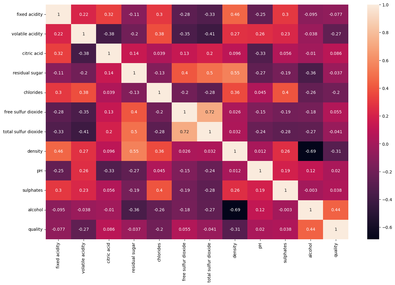
alcohol is most highly correlated with quality. Looking for other informative features, notice that volatile acidity correlates with quality but not with alcohol, making it a good second feature. Remember that a correlation matrix is not helpful if predictive signals are encoded in combinations of features.
42.88.3. Validate Input Data against Data Schema#
Before processing your data, you should validate the data against a data schema as described in Data and Feature Debugging.
First, define a function that validates data against a schema.
#@title Define function to validate data

def test_data_schema(input_data, schema):
  """Tests that the datatypes and ranges of values in the dataset
    adhere to expectations.

    Args:
      input_function: Dataframe containing data to test
      schema: Schema which describes the properties of the data.
  """

  def test_dtypes():
    for column in schema.keys():
      assert input_data[column].map(type).eq(
          schema[column]['dtype']).all(), (
          "Incorrect dtype in column '%s'." % column
      )
    print('Input dtypes are correct.')

  def test_ranges():
    for column in schema.keys():
      schema_max = schema[column]['range']['max']
      schema_min = schema[column]['range']['min']
      # Assert that data falls between schema min and max.
      assert input_data[column].max() <= schema_max, (
          "Maximum value of column '%s' is too low." % column
      )
      assert input_data[column].min() >= schema_min, (
          "Minimum value of column '%s' is too high." % column
      )
    print('Data falls within specified ranges.')

  test_dtypes()
  test_ranges()
To define your schema, you need to understand the statistical properties of your dataset. Generate statistics on your dataset by running the following code cell:
wineDf.describe()
| fixed acidity | volatile acidity | citric acid | residual sugar | chlorides | free sulfur dioxide | total sulfur dioxide | density | pH | sulphates | alcohol | quality | |
|---|---|---|---|---|---|---|---|---|---|---|---|---|
| count | 6497.0 | 6497.0 | 6497.0 | 6497.0 | 6497.0 | 6497.0 | 6497.0 | 6497.0 | 6497.0 | 6497.0 | 6497.0 | 6497.0 |
| mean | 7.2 | 0.3 | 0.3 | 5.4 | 0.1 | 30.5 | 115.7 | 1.0 | 3.2 | 0.5 | 10.5 | 5.8 |
| std | 1.3 | 0.2 | 0.1 | 4.8 | 0.0 | 17.7 | 56.5 | 0.0 | 0.2 | 0.1 | 1.2 | 0.9 |
| min | 3.8 | 0.1 | 0.0 | 0.6 | 0.0 | 1.0 | 6.0 | 1.0 | 2.7 | 0.2 | 8.0 | 3.0 |
| 25% | 6.4 | 0.2 | 0.2 | 1.8 | 0.0 | 17.0 | 77.0 | 1.0 | 3.1 | 0.4 | 9.5 | 5.0 |
| 50% | 7.0 | 0.3 | 0.3 | 3.0 | 0.0 | 29.0 | 118.0 | 1.0 | 3.2 | 0.5 | 10.3 | 6.0 |
| 75% | 7.7 | 0.4 | 0.4 | 8.1 | 0.1 | 41.0 | 156.0 | 1.0 | 3.3 | 0.6 | 11.3 | 6.0 |
| max | 15.9 | 1.6 | 1.7 | 65.8 | 0.6 | 289.0 | 440.0 | 1.0 | 4.0 | 2.0 | 14.9 | 9.0 |
Using the statistics generated above, define the data schema in the following code cell. For demonstration purposes, restrict your data schema to the first three data columns. For each data column, enter the:
minimum value
maximum value
data type
As an example, the values for the first column are filled out. After entering the values, run the code cell to confirm that your input data matches the schema.
wine_schema = {
    'fixed acidity': {
        'range': {
            'min': 3.8,
            'max': 15.9
        },
        'dtype': float,
    },
    'volatile acidity': {
        'range': {
            'min': 0.08,  # Placeholder value, update with the actual minimum
            'max': 1.58  # Placeholder value, update with the actual maximum
        },
        'dtype': float,  # Placeholder value, update with the actual dtype
    },
    'citric acid': {
        'range': {
            'min': 0.0,  # Placeholder value, update with the actual minimum
            'max': 1.66  # Placeholder value, update with the actual maximum
        },
        'dtype': float,  # Placeholder value, update with the actual dtype
    }
}

print('Validating wine data against data schema...')
test_data_schema(wineDf, wine_schema)
Validating wine data against data schema...
Input dtypes are correct.
Data falls within specified ranges.
42.88.3.1. Solution#
wine_schema = {
    'fixed acidity': {
        'range': {
            'min': 3.7,
            'max': 15.9
        },
        'dtype': float,
    },
    'volatile acidity': {
        'range': {
            'min': 0.08,  # minimum value
            'max': 1.6   # maximum value
        },
        'dtype': float,    # data type
    },
    'citric acid': {
        'range': {
            'min': 0.0, # minimum value
            'max': 1.7  # maximum value
        },
        'dtype': float,   # data type
    }
}

print('Validating wine data against data schema...')
test_data_schema(wineDf, wine_schema)
Validating wine data against data schema...
Input dtypes are correct.
Data falls within specified ranges.
42.88.4. Split and Normalize Data#
Split the dataset into data and labels.
wineFeatures = wineDf.copy(deep=True)
wineFeatures.drop(columns='quality',inplace=True)
wineLabels = wineDf['quality'].copy(deep=True)
Normalize data using z-score.
def normalizeData(arr):
  stdArr = np.std(arr)
  meanArr = np.mean(arr)
  arr = (arr-meanArr)/stdArr
  return arr

for str1 in wineFeatures.columns:
   wineFeatures[str1] = normalizeData(wineFeatures[str1])
42.88.5. Test Engineered Data#
After normalizing your data, you should test your engineered data for errors as described in Data and Feature Debugging. In this section, you will test that engineering data:
Has the expected number of rows and columns.
Does not have null values.
First, set up the testing functions by running the following code cell:
import unittest

def test_input_dim(df, n_rows, n_columns):
  assert len(df) == n_rows, "Unexpected number of rows."
  assert len(df.columns) == n_columns, "Unexpected number of columns."
  print('Engineered data has the expected number of rows and columns.')

def test_nulls(df):
  dataNulls = df.isnull().sum().sum()
  assert dataNulls == 0, "Nulls in engineered data."
  print('Engineered features do not contain nulls.')
Your input data had 6497 examples and 11 feature columns. Test whether your engineered data has the expected number of rows and columns by running the following cell. Confirm that the test fails if you change the values below.
#@title Test dimensions of engineered data
wine_feature_rows = 6497 #@param
wine_feature_cols = 11 #@param
test_input_dim(wineFeatures,
               wine_feature_rows,
               wine_feature_cols)
Engineered data has the expected number of rows and columns.
Test that your engineered data does not contain nulls by running the code below.
test_nulls(wineFeatures)
Engineered features do not contain nulls.
42.88.6. Check Splits for Statistical Equivalence#
As described in the Data Debugging guidelines, before developing your model, you should check that your training and validation splits are equally representative. Assuming a training:validation split of 80:20, compare the mean and the standard deviation of the splits by running the next two code cells. Note that this comparison is not a rigorous test for statistical equivalence but simply a quick and dirty comparison of the splits.
splitIdx = int(wineFeatures.shape[0] * 8 / 10)
wineFeatures.iloc[0:splitIdx, :].describe()
| fixed acidity | volatile acidity | citric acid | residual sugar | chlorides | free sulfur dioxide | total sulfur dioxide | density | pH | sulphates | alcohol | |
|---|---|---|---|---|---|---|---|---|---|---|---|
| count | 5197.0 | 5197.0 | 5197.0 | 5197.0 | 5197.0 | 5197.0 | 5197.0 | 5197.0 | 5197.0 | 5197.0 | 5197.0 |
| mean | -0.2 | -0.3 | 0.1 | 0.2 | -0.2 | 0.2 | 0.3 | -0.2 | -0.1 | -0.2 | -0.0 |
| std | 0.7 | 0.8 | 0.9 | 1.1 | 0.9 | 1.0 | 0.8 | 1.0 | 1.0 | 0.9 | 1.0 |
| min | -2.6 | -1.6 | -2.2 | -1.0 | -1.3 | -1.6 | -1.9 | -2.5 | -3.1 | -2.1 | -2.1 |
| 25% | -0.7 | -0.8 | -0.4 | -0.8 | -0.6 | -0.5 | -0.2 | -1.0 | -0.8 | -0.8 | -0.9 |
| 50% | -0.3 | -0.4 | -0.1 | -0.1 | -0.3 | 0.1 | 0.3 | -0.2 | -0.2 | -0.3 | -0.2 |
| 75% | 0.1 | 0.0 | 0.5 | 0.9 | -0.1 | 0.8 | 0.9 | 0.6 | 0.4 | 0.2 | 0.7 |
| max | 6.0 | 6.0 | 9.2 | 12.7 | 15.8 | 14.6 | 5.7 | 14.8 | 4.2 | 9.9 | 3.1 |
wineFeatures.iloc[splitIdx:-1,:].describe()
| fixed acidity | volatile acidity | citric acid | residual sugar | chlorides | free sulfur dioxide | total sulfur dioxide | density | pH | sulphates | alcohol | |
|---|---|---|---|---|---|---|---|---|---|---|---|
| count | 1299.0 | 1299.0 | 1299.0 | 1299.0 | 1299.0 | 1299.0 | 1299.0 | 1299.0 | 1299.0 | 1299.0 | 1299.0 |
| mean | 0.9 | 1.1 | -0.3 | -0.6 | 0.8 | -0.8 | -1.3 | 0.7 | 0.6 | 0.8 | 0.0 |
| std | 1.4 | 1.1 | 1.3 | 0.3 | 1.1 | 0.6 | 0.6 | 0.7 | 1.0 | 1.0 | 0.9 |
| min | -1.8 | -1.3 | -2.2 | -1.0 | -1.3 | -1.7 | -1.9 | -1.5 | -2.2 | -1.1 | -1.8 |
| 25% | -0.1 | 0.3 | -1.5 | -0.7 | 0.4 | -1.3 | -1.7 | 0.3 | -0.1 | 0.1 | -0.7 |
| 50% | 0.6 | 1.0 | -0.3 | -0.7 | 0.7 | -0.9 | -1.4 | 0.7 | 0.5 | 0.6 | -0.1 |
| 75% | 1.7 | 1.8 | 0.8 | -0.6 | 1.0 | -0.5 | -1.0 | 1.1 | 1.1 | 1.3 | 0.7 |
| max | 6.7 | 7.5 | 3.2 | 2.1 | 10.4 | 2.3 | 3.1 | 3.0 | 4.9 | 7.3 | 3.7 |
The two splits are clearly not equally representative. To make the splits equally representative, you can shuffle the data.
Run the following code cell to shuffle the data, and then recreate the features and labels from the shuffled data.
# Shuffle data
wineDf = wineDf.sample(frac=1).reset_index(drop=True)
# Recreate features and labels
wineFeatures = wineDf.copy(deep=True)
wineFeatures.drop(columns='quality',inplace=True)
wineLabels = wineDf['quality'].copy(deep=True)
Now, confirm that the splits are equally representative by regenerating and comparing the statistics using the previous code cells. You may wonder why the initial splits differed so greatly. It turns out that in the wine dataset, the first 4897 rows contain data on white wines and the next 1599 rows contain data on red wines. When you split your dataset 80:20, then your training dataset contains 5197 examples, which is 94% white wine. The validation dataset is purely red wine.
Ensuring your splits are statistically equivalent is a good development practice. In general, following good development practices will simplify your model debugging. To learn about testing for statistical equivalence, see Equivalence Tests Lakens, D..
42.88.7. Establish a Baseline#
For a regression problem, the simplest baseline to predict the average value. Run the following code to calculate the mean-squared error (MSE) loss on the training split using the average value as a baseline. Your loss is approximately 0.75. Any model should beat this loss to justify its use.
baselineMSE = np.square(wineLabels[0:splitIdx]-np.mean(wineLabels[0:splitIdx]))
baselineMSE = np.sum(baselineMSE)/len(baselineMSE)
print(baselineMSE)
0.7738266430037695
42.88.8. Linear Model#
Following good ML dev practice, let’s start with a linear model that uses the most informative feature from the correlation matrix: alcohol. Even if this model performs badly, we can still use it as a baseline. This model should beat our previous baseline’s MSE of 0.75.
First, let’s define a function to plot our loss and accuracy curves. The function will also print the final loss and accuracy. Instead of using verbose=1, you can call the function.
def showRegressionResults(trainHistory):
  """Function to:
   * Print final loss.
   * Plot loss curves.

  Args:
    trainHistory: object returned by model.fit
  """

  # Print final loss
  print("Final training loss: " + str(trainHistory.history['loss'][-1]))
  print("Final Validation loss: " + str(trainHistory.history['val_loss'][-1]))

  # Plot loss curves
  plt.plot(trainHistory.history['loss'])
  plt.plot(trainHistory.history['val_loss'])
  plt.legend(['Training loss','Validation loss'],loc='best')
  plt.title('Loss Curves')
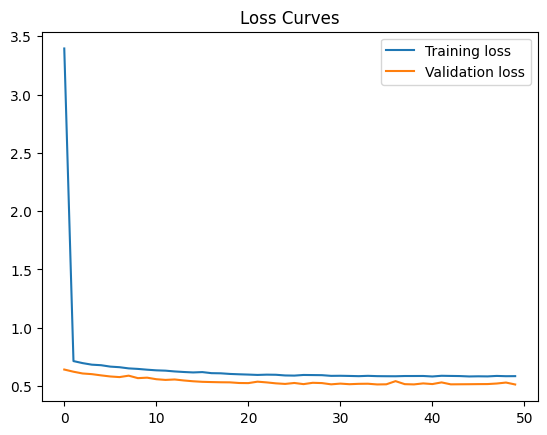
For fast prototyping, let’s try using a full batch per epoch to update the gradient only once per epoch. Use the full batch by setting batch_size = wineFeatures.shape[0] as indicated by the code comment.
What do you think of the loss curve? Can you improve it? For hints and discussion, see the following text cells.
model = None
# Choose feature
wineFeaturesSimple = wineFeatures['alcohol']
# Define model
model = keras.Sequential()
model.add(keras.layers.Dense(units=1, activation='linear', input_dim=1))
# Specify the optimizer using the TF API to specify the learning rate
model.compile(optimizer=tf.optimizers.Adam(learning_rate=0.01),
              loss='mse')
# Train the model!
trainHistory = model.fit(wineFeaturesSimple,
                         wineLabels,
                         epochs=50,
                         batch_size=32,  # Replace with your desired batch size
                         validation_split=0.2,
                         verbose=0)
# Plot
showRegressionResults(trainHistory)
Final training loss: 0.6339302659034729
Final Validation loss: 0.5759974718093872
42.88.8.1. Hint#
The loss decreases but very slowly. Possible fixes are:
Increase number of epochs.
Increase learning rate.
Decrease batch size. A lower batch size can result in larger decrease in loss per epoch, under the assumption that the smaller batches stay representative of the overall data distribution.
Play with these three parameters in the code above to decrease the loss.
42.88.8.2. Solution#
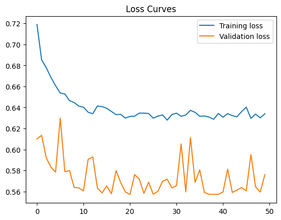
Run the following code cell to train the model using a reduced batch size of 100. Reducing the batch size leads to a greater decrease in loss per epoch. The minimum achievable loss is about 0.64. This is a significant increase over our baseline of 0.75.
model = None
# Choose feature
wineFeaturesSimple = wineFeatures['alcohol']
# Define model
model = keras.Sequential()
model.add(keras.layers.Dense(units=1, activation='linear', input_dim=1))
# Specify the optimizer using the TF API to specify the learning rate
model.compile(optimizer=tf.optimizers.Adam(learning_rate=0.01),
              loss='mse')
# Train the model!
trainHistory = model.fit(wineFeaturesSimple,
                         wineLabels,
                         epochs=20,
                         batch_size=100, # set batch size here
                         validation_split=0.2,
                         verbose=0)
# Plot
showRegressionResults(trainHistory)
Final training loss: 0.6591692566871643
Final Validation loss: 0.5836994051933289
42.88.9. Add Feature to Linear Model#
Try adding a feature to the linear model. Since you need to combine the two features into one prediction for regression, you’ll also need to add a second layer. Modify the code below to implement the following changes:
Add
'volatile acidity'to the features inwineFeaturesSimple.Add a second linear layer with 1 unit.
Experiment with learning rate, epochs, and batch_size to try to reduce loss.
What happens to your loss?
model = None
# Select features
wineFeaturesSimple = wineFeatures[['alcohol', 'volatile acidity']]  # Add other features as needed
# Define model
model = keras.Sequential()
model.add(keras.layers.Dense(wineFeaturesSimple.shape[1],
                             input_dim=wineFeaturesSimple.shape[1],
                             activation='linear'))

# Compile
model.compile(optimizer=tf.optimizers.Adam(learning_rate=0.01),  # Replace with your desired learning rate
              loss='mse')
# Train
trainHistory = model.fit(wineFeaturesSimple,
                         wineLabels,
                         epochs=50,  # Replace with your desired number of epochs
                         batch_size=32,  # Replace with your desired batch size
                         validation_split=0.2,
                         verbose=0)
# Plot results
showRegressionResults(trainHistory)
Final training loss: 0.5843960046768188
Final Validation loss: 0.5128785371780396

42.88.9.1. Solution#
Run the following code to add the second feature and the second layer. The training loss is about 0.59, a small decrease from the previous loss of 0.64.
model = None
# Select features
wineFeaturesSimple = wineFeatures[['alcohol', 'volatile acidity']] # add second feature
# Define model
model = keras.Sequential()
model.add(keras.layers.Dense(wineFeaturesSimple.shape[1],
                             input_dim=wineFeaturesSimple.shape[1],
                             activation='linear'))
model.add(keras.layers.Dense(1, activation='linear')) # add second layer
# Compile
model.compile(optimizer=tf.optimizers.Adam(learning_rate=0.01), loss='mse')
# Train
trainHistory = model.fit(wineFeaturesSimple,
                         wineLabels,
                         epochs=20,
                         batch_size=100,
                         validation_split=0.2,
                         verbose=0)
# Plot results
showRegressionResults(trainHistory)
Final training loss: 0.5994521975517273
Final Validation loss: 0.5335853695869446
42.88.10. Use a Nonlinear Model#
Let’s try a nonlinear model. Modify the code below to make the following changes:
Change the first layer to use
relu. (Output layer stays linear since this is a regression problem.)As usual, specify the learning rate, epochs, and batch_size.
Run the cell. Does the loss increase, decrease, or stay the same?
model = None
# Define
model = keras.Sequential()
model.add(keras.layers.Dense(units=wineFeaturesSimple.shape[1],
                             input_dim=wineFeaturesSimple.shape[1],
                             activation='relu'))  # Replace 'relu' with your desired activation function
model.add(keras.layers.Dense(units=1, activation='linear'))
# Compile
model.compile(optimizer=tf.optimizers.Adam(), loss='mse')
# Fit
model.fit(wineFeaturesSimple,
          wineLabels,
          epochs=50,  # Replace with your desired number of epochs
          batch_size=32,  # Replace with your desired batch size
          validation_split=0.2,
          verbose=0)
# Plot results
showRegressionResults(trainHistory)
Final training loss: 0.5843960046768188
Final Validation loss: 0.5128785371780396
42.88.10.1. Solution#
Run the following cell to use a relu activation in your first hidden layer. Your loss stays about the same, perhaps declining negligibly to 0.58.
model = None
# Define
model = keras.Sequential()
model.add(keras.layers.Dense(wineFeaturesSimple.shape[1],
                             input_dim=wineFeaturesSimple.shape[1],
                             activation='relu'))
model.add(keras.layers.Dense(1, activation='linear'))
# Compile
model.compile(optimizer=tf.optimizers.Adam(), loss='mse')
# Fit
model.fit(wineFeaturesSimple,
          wineLabels,
          epochs=20,
          batch_size=100,
          validation_split=0.2,
          verbose=0)
# Plot results
showRegressionResults(trainHistory)
Final training loss: 0.5843960046768188
Final Validation loss: 0.5128785371780396

42.88.11. Optimize Your Model#
We have two features with one hidden layer but didn’t see an improvement. At this point, it’s tempting to use all your features with a high-capacity network. However, you must resist the temptation. Instead, follow the guidance in Model Optimization to improve model performance. For a hint and for a discussion, see the following text sections.
# Choose features
wineFeaturesSimple = wineFeatures[['alcohol', 'volatile acidity']] # add features

# Define
model = None
model = keras.Sequential()
model.add(keras.layers.Dense(wineFeaturesSimple.shape[1],
                             activation='relu',
                             input_dim=wineFeaturesSimple.shape[1]))

# Add more layers here
model.add(keras.layers.Dense(1, activation='linear'))

# Compile
model.compile(optimizer=tf.optimizers.Adam(), loss='mse')

# Train
trainHistory = model.fit(wineFeaturesSimple,
                         wineLabels,
                         epochs=50,  # Replace with your desired number of epochs
                         batch_size=32,  # Replace with your desired batch size
                         validation_split=0.2,
                         verbose=0)

# Plot results
showRegressionResults(trainHistory)
Final training loss: 0.7648102045059204
Final Validation loss: 0.7018823027610779
42.88.11.1. Hint#
You can try to reduce loss by adding features, adding layers, or playing with the hyperparameters. Before adding more features, check the correlation matrix. Don’t expect your loss to decrease by much. Sadly, that is a common experience in machine learning!
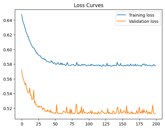
42.88.11.2. Solution#
Run the following code to:
Add the features chlorides and density.
Set training epochs to 100.
Set batch size to 100.
Your loss reduces to about 0.56. That’s a minor improvement over the previous loss of 0.58. It seems that adding more features or capacity isn’t improving your model by much. Perhaps your model has a bug? In the next section, you will run a sanity check on your model.
# Choose features
wineFeaturesSimple = wineFeatures[['alcohol','volatile acidity','chlorides','density']]
# Define
model = None
model = keras.Sequential()
model.add(keras.layers.Dense(wineFeaturesSimple.shape[1],
                             activation='relu',
                             input_dim=wineFeaturesSimple.shape[1]))
# Add more layers here
model.add(keras.layers.Dense(1,activation='linear'))
# Compile
model.compile(optimizer=tf.optimizers.Adam(), loss='mse')
# Train
trainHistory = model.fit(wineFeaturesSimple,
                         wineLabels,
                         epochs=200,
                         batch_size=100,
                         validation_split=0.2,
                         verbose=0)
# Plot results
showRegressionResults(trainHistory)
Final training loss: 0.5778111219406128
Final Validation loss: 0.51249098777771
42.88.12. Check for Implementation Bugs using Reduced Dataset#
Your loss isn’t decreasing by much. Perhaps your model has an implementation bug. From the Model Debugging guidelines, a quick test for implementation bugs is to obtain a low loss on a reduced dataset of, say, 10 examples. Remember, passing this test does not validate your modeling approach but only checks for basic implementation bugs. In your ML problem, if your model passes this test, then continue debugging your model to train on your full dataset.
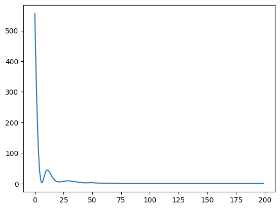
In the following code, experiment with the learning rate, batch size, and number of epochs. Can you reach a low loss? Choose hyperparameter values that let you iterate quickly.
# Choose 10 examples
wineFeaturesSmall = wineFeatures[0:10]
wineLabelsSmall = wineLabels[0:10]

# Define model
model = None
model = keras.Sequential()
model.add(keras.layers.Dense(wineFeaturesSmall.shape[1],
                             activation='relu',
                             input_dim=wineFeaturesSmall.shape[1]))
model.add(keras.layers.Dense(wineFeaturesSmall.shape[1], activation='relu'))
model.add(keras.layers.Dense(1, activation='linear'))

# Compile
model.compile(optimizer=tf.optimizers.Adam(), loss='mse')  # Set learning rate

# Train
trainHistory = model.fit(wineFeaturesSmall,
                        wineLabelsSmall,
                        epochs=50,  # Replace with your desired number of epochs
                        batch_size=32,  # Replace with your desired batch size
                        verbose=0)

# Plot results
print("Final training loss: " + str(trainHistory.history['loss'][-1]))
plt.plot(trainHistory.history['loss'])
Final training loss: 11.7090482711792
[<matplotlib.lines.Line2D at 0x7e3d355e1e70>]
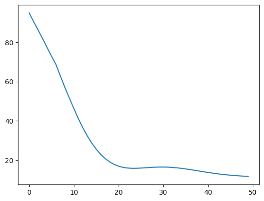
42.88.12.1. Solution#
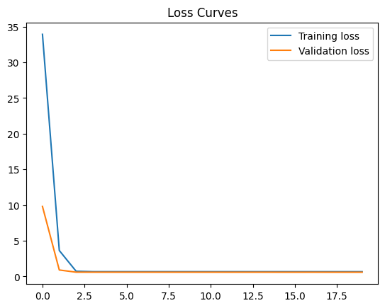
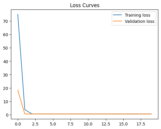
Run the following code cell to train the model using these hyperparameter values:
learning rate = 0.01
epochs = 200
batch size = 10
You get a low loss on your reduced dataset. This result means your model is probably solid and your previous results are as good as they’ll get.
# Choose 10 examples
wineFeaturesSmall = wineFeatures[0:10]
wineLabelsSmall = wineLabels[0:10]
# Define model
model = None
model = keras.Sequential()
model.add(keras.layers.Dense(wineFeaturesSmall.shape[1], activation='relu',
                             input_dim=wineFeaturesSmall.shape[1]))
model.add(keras.layers.Dense(wineFeaturesSmall.shape[1], activation='relu'))
model.add(keras.layers.Dense(1, activation='linear'))
# Compile
model.compile(optimizer=tf.optimizers.Adam(0.01), loss='mse') # set LR
# Train
trainHistory = model.fit(wineFeaturesSmall,
                        wineLabelsSmall,
                        epochs=200,
                        batch_size=10,
                        verbose=0)
# Plot results
print("Final training loss: " + str(trainHistory.history['loss'][-1]))
plt.plot(trainHistory.history['loss'])
Final training loss: 0.33318591117858887
[<matplotlib.lines.Line2D at 0x7e3d441045e0>]
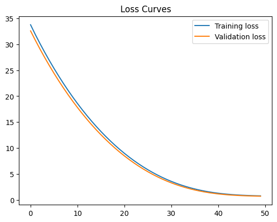
42.88.13. Trying a Very Complex Model#
Let’s go all in and use a very complex model with all the features. For science! And to satisfy ourselves that a simple model is indeed better. Let’s use all 11 features with 3 fully-connected relu layers and a final linear layer. The next cell takes a while to run. Skip to the results in the cell after if you like.
model = None
# Define
model = keras.Sequential()
model.add(keras.layers.Dense(wineFeatures.shape[1], activation='relu',
                             input_dim=wineFeatures.shape[1]))
model.add(keras.layers.Dense(wineFeatures.shape[1], activation='relu'))
model.add(keras.layers.Dense(wineFeatures.shape[1], activation='relu'))
model.add(keras.layers.Dense(1,activation='linear'))
# Compile
model.compile(optimizer=tf.optimizers.Adam(), loss='mse')
# Train the model!
trainHistory = model.fit(wineFeatures, wineLabels, epochs=100, batch_size=100,
                         verbose=1, validation_split = 0.2)
# Plot results
showRegressionResults(trainHistory)
plt.ylim(0.4,1)
Epoch 1/100
52/52 [==============================] - 1s 8ms/step - loss: 10.1107 - val_loss: 5.9102
Epoch 2/100
52/52 [==============================] - 0s 4ms/step - loss: 5.0580 - val_loss: 4.2809
Epoch 3/100
52/52 [==============================] - 0s 4ms/step - loss: 3.0781 - val_loss: 1.6974
Epoch 4/100
52/52 [==============================] - 0s 5ms/step - loss: 1.5744 - val_loss: 1.0843
Epoch 5/100
52/52 [==============================] - 0s 5ms/step - loss: 1.1691 - val_loss: 0.8313
Epoch 6/100
52/52 [==============================] - 0s 5ms/step - loss: 0.9342 - val_loss: 0.7203
Epoch 7/100
52/52 [==============================] - 0s 3ms/step - loss: 0.8001 - val_loss: 0.6452
Epoch 8/100
52/52 [==============================] - 0s 3ms/step - loss: 0.7394 - val_loss: 0.5998
Epoch 9/100
52/52 [==============================] - 0s 3ms/step - loss: 0.6811 - val_loss: 0.5844
Epoch 10/100
52/52 [==============================] - 0s 2ms/step - loss: 0.6714 - val_loss: 0.5682
Epoch 11/100
52/52 [==============================] - 0s 3ms/step - loss: 0.6571 - val_loss: 0.5636
Epoch 12/100
52/52 [==============================] - 0s 3ms/step - loss: 0.6560 - val_loss: 0.5587
Epoch 13/100
52/52 [==============================] - 0s 3ms/step - loss: 0.6351 - val_loss: 0.5630
Epoch 14/100
52/52 [==============================] - 0s 3ms/step - loss: 0.6233 - val_loss: 0.5414
Epoch 15/100
52/52 [==============================] - 0s 3ms/step - loss: 0.6215 - val_loss: 0.5577
Epoch 16/100
52/52 [==============================] - 0s 3ms/step - loss: 0.6176 - val_loss: 0.5470
Epoch 17/100
52/52 [==============================] - 0s 3ms/step - loss: 0.6180 - val_loss: 0.5335
Epoch 18/100
52/52 [==============================] - 0s 3ms/step - loss: 0.6123 - val_loss: 0.5459
Epoch 19/100
52/52 [==============================] - 0s 3ms/step - loss: 0.6090 - val_loss: 0.5325
Epoch 20/100
52/52 [==============================] - 0s 3ms/step - loss: 0.6000 - val_loss: 0.5298
Epoch 21/100
52/52 [==============================] - 0s 3ms/step - loss: 0.5983 - val_loss: 0.5214
Epoch 22/100
52/52 [==============================] - 0s 3ms/step - loss: 0.5977 - val_loss: 0.5245
Epoch 23/100
52/52 [==============================] - 0s 3ms/step - loss: 0.5999 - val_loss: 0.5583
Epoch 24/100
52/52 [==============================] - 0s 3ms/step - loss: 0.5969 - val_loss: 0.5317
Epoch 25/100
52/52 [==============================] - 0s 2ms/step - loss: 0.6043 - val_loss: 0.5147
Epoch 26/100
52/52 [==============================] - 0s 3ms/step - loss: 0.5909 - val_loss: 0.5159
Epoch 27/100
52/52 [==============================] - 0s 2ms/step - loss: 0.5897 - val_loss: 0.5121
Epoch 28/100
52/52 [==============================] - 0s 2ms/step - loss: 0.5932 - val_loss: 0.5663
Epoch 29/100
52/52 [==============================] - 0s 3ms/step - loss: 0.5919 - val_loss: 0.5229
Epoch 30/100
52/52 [==============================] - 0s 3ms/step - loss: 0.5835 - val_loss: 0.5169
Epoch 31/100
52/52 [==============================] - 0s 2ms/step - loss: 0.5797 - val_loss: 0.5089
Epoch 32/100
52/52 [==============================] - 0s 3ms/step - loss: 0.5781 - val_loss: 0.5065
Epoch 33/100
52/52 [==============================] - 0s 3ms/step - loss: 0.5766 - val_loss: 0.5060
Epoch 34/100
52/52 [==============================] - 0s 3ms/step - loss: 0.5791 - val_loss: 0.5149
Epoch 35/100
52/52 [==============================] - 0s 3ms/step - loss: 0.5989 - val_loss: 0.5289
Epoch 36/100
52/52 [==============================] - 0s 3ms/step - loss: 0.6003 - val_loss: 0.5356
Epoch 37/100
52/52 [==============================] - 0s 3ms/step - loss: 0.5821 - val_loss: 0.5042
Epoch 38/100
52/52 [==============================] - 0s 3ms/step - loss: 0.5719 - val_loss: 0.5030
Epoch 39/100
52/52 [==============================] - 0s 3ms/step - loss: 0.5781 - val_loss: 0.5014
Epoch 40/100
52/52 [==============================] - 0s 3ms/step - loss: 0.5758 - val_loss: 0.5395
Epoch 41/100
52/52 [==============================] - 0s 3ms/step - loss: 0.5741 - val_loss: 0.5062
Epoch 42/100
52/52 [==============================] - 0s 3ms/step - loss: 0.5726 - val_loss: 0.5127
Epoch 43/100
52/52 [==============================] - 0s 2ms/step - loss: 0.5683 - val_loss: 0.5002
Epoch 44/100
52/52 [==============================] - 0s 2ms/step - loss: 0.5734 - val_loss: 0.5106
Epoch 45/100
52/52 [==============================] - 0s 3ms/step - loss: 0.5713 - val_loss: 0.5118
Epoch 46/100
52/52 [==============================] - 0s 3ms/step - loss: 0.5906 - val_loss: 0.4978
Epoch 47/100
52/52 [==============================] - 0s 3ms/step - loss: 0.5761 - val_loss: 0.5143
Epoch 48/100
52/52 [==============================] - 0s 3ms/step - loss: 0.5636 - val_loss: 0.5006
Epoch 49/100
52/52 [==============================] - 0s 3ms/step - loss: 0.5736 - val_loss: 0.5068
Epoch 50/100
52/52 [==============================] - 0s 3ms/step - loss: 0.5643 - val_loss: 0.5086
Epoch 51/100
52/52 [==============================] - 0s 3ms/step - loss: 0.5614 - val_loss: 0.4964
Epoch 52/100
52/52 [==============================] - 0s 3ms/step - loss: 0.5792 - val_loss: 0.4966
Epoch 53/100
52/52 [==============================] - 0s 3ms/step - loss: 0.5697 - val_loss: 0.5660
Epoch 54/100
52/52 [==============================] - 0s 3ms/step - loss: 0.5816 - val_loss: 0.4941
Epoch 55/100
52/52 [==============================] - 0s 3ms/step - loss: 0.5679 - val_loss: 0.5029
Epoch 56/100
52/52 [==============================] - 0s 2ms/step - loss: 0.5675 - val_loss: 0.4994
Epoch 57/100
52/52 [==============================] - 0s 2ms/step - loss: 0.5618 - val_loss: 0.4932
Epoch 58/100
52/52 [==============================] - 0s 2ms/step - loss: 0.5676 - val_loss: 0.4896
Epoch 59/100
52/52 [==============================] - 0s 3ms/step - loss: 0.5602 - val_loss: 0.4893
Epoch 60/100
52/52 [==============================] - 0s 3ms/step - loss: 0.5555 - val_loss: 0.5295
Epoch 61/100
52/52 [==============================] - 0s 3ms/step - loss: 0.5677 - val_loss: 0.5429
Epoch 62/100
52/52 [==============================] - 0s 3ms/step - loss: 0.5622 - val_loss: 0.4897
Epoch 63/100
52/52 [==============================] - 0s 3ms/step - loss: 0.5732 - val_loss: 0.4886
Epoch 64/100
52/52 [==============================] - 0s 3ms/step - loss: 0.5670 - val_loss: 0.4880
Epoch 65/100
52/52 [==============================] - 0s 2ms/step - loss: 0.5759 - val_loss: 0.4933
Epoch 66/100
52/52 [==============================] - 0s 3ms/step - loss: 0.5702 - val_loss: 0.5184
Epoch 67/100
52/52 [==============================] - 0s 3ms/step - loss: 0.5570 - val_loss: 0.4869
Epoch 68/100
52/52 [==============================] - 0s 3ms/step - loss: 0.5545 - val_loss: 0.4860
Epoch 69/100
52/52 [==============================] - 0s 3ms/step - loss: 0.5596 - val_loss: 0.4951
Epoch 70/100
52/52 [==============================] - 0s 3ms/step - loss: 0.5811 - val_loss: 0.5845
Epoch 71/100
52/52 [==============================] - 0s 3ms/step - loss: 0.5685 - val_loss: 0.4868
Epoch 72/100
52/52 [==============================] - 0s 3ms/step - loss: 0.5553 - val_loss: 0.4904
Epoch 73/100
52/52 [==============================] - 0s 3ms/step - loss: 0.5569 - val_loss: 0.4846
Epoch 74/100
52/52 [==============================] - 0s 3ms/step - loss: 0.5619 - val_loss: 0.4842
Epoch 75/100
52/52 [==============================] - 0s 3ms/step - loss: 0.5606 - val_loss: 0.4840
Epoch 76/100
52/52 [==============================] - 0s 4ms/step - loss: 0.5609 - val_loss: 0.5185
Epoch 77/100
52/52 [==============================] - 0s 4ms/step - loss: 0.5972 - val_loss: 0.4855
Epoch 78/100
52/52 [==============================] - 0s 4ms/step - loss: 0.5677 - val_loss: 0.4825
Epoch 79/100
52/52 [==============================] - 0s 4ms/step - loss: 0.5563 - val_loss: 0.4875
Epoch 80/100
52/52 [==============================] - 0s 3ms/step - loss: 0.5526 - val_loss: 0.4960
Epoch 81/100
52/52 [==============================] - 0s 4ms/step - loss: 0.5552 - val_loss: 0.5070
Epoch 82/100
52/52 [==============================] - 0s 4ms/step - loss: 0.5535 - val_loss: 0.4903
Epoch 83/100
52/52 [==============================] - 0s 4ms/step - loss: 0.5566 - val_loss: 0.5203
Epoch 84/100
52/52 [==============================] - 0s 4ms/step - loss: 0.5538 - val_loss: 0.4860
Epoch 85/100
52/52 [==============================] - 0s 3ms/step - loss: 0.5700 - val_loss: 0.5153
Epoch 86/100
52/52 [==============================] - 0s 4ms/step - loss: 0.5555 - val_loss: 0.4886
Epoch 87/100
52/52 [==============================] - 0s 4ms/step - loss: 0.5510 - val_loss: 0.4816
Epoch 88/100
52/52 [==============================] - 0s 4ms/step - loss: 0.5529 - val_loss: 0.4927
Epoch 89/100
52/52 [==============================] - 0s 4ms/step - loss: 0.5492 - val_loss: 0.4852
Epoch 90/100
52/52 [==============================] - 0s 4ms/step - loss: 0.5496 - val_loss: 0.4937
Epoch 91/100
52/52 [==============================] - 0s 4ms/step - loss: 0.5633 - val_loss: 0.4809
Epoch 92/100
52/52 [==============================] - 0s 4ms/step - loss: 0.5701 - val_loss: 0.5083
Epoch 93/100
52/52 [==============================] - 0s 4ms/step - loss: 0.5765 - val_loss: 0.5725
Epoch 94/100
52/52 [==============================] - 0s 3ms/step - loss: 0.5581 - val_loss: 0.4898
Epoch 95/100
52/52 [==============================] - 0s 2ms/step - loss: 0.5595 - val_loss: 0.5327
Epoch 96/100
52/52 [==============================] - 0s 2ms/step - loss: 0.5616 - val_loss: 0.5250
Epoch 97/100
52/52 [==============================] - 0s 3ms/step - loss: 0.5724 - val_loss: 0.4854
Epoch 98/100
52/52 [==============================] - 0s 3ms/step - loss: 0.5451 - val_loss: 0.5053
Epoch 99/100
52/52 [==============================] - 0s 3ms/step - loss: 0.5511 - val_loss: 0.5023
Epoch 100/100
52/52 [==============================] - 0s 3ms/step - loss: 0.5540 - val_loss: 0.4844
Final training loss: 0.5540224313735962
Final Validation loss: 0.48444509506225586
(0.4, 1.0)
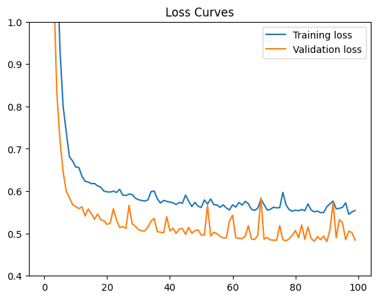
42.88.13.1. Results#
If you train for long enough, the minimum achievable MSE is around 0.52, which is a decrease of 0.04 from the previous best loss of 0.56. This decrease probably isn’t worth the performance and complexity cost of using all your features and a deeper network. However, that decision depends on the objectives you’re optimizing for.
If you train the model long enough, the validation loss actually starts increasing while training loss continues to decrease. This divergence in loss curves means your model is overfitting. The overfitting results from the closer fit that your very complex model can learn. Stick with the simpler model. You’ll be happier and live longer!
If you do want to optimize your loss, then play with the model to find the minimum achievable training loss before overfitting sets in. Try playing with the network parameters in the code cell above to achieve a loss of 0.51. But be warned—optimizing your loss could take a lot of trial and error…
42.88.14. Conclusion#
This Colab demonstrated the following principles:
The most important step in machine learning is understanding your data.
The largest gains come from the initial features and network.
Returns diminish as you add features and complexity.
Incremental development provides confidence in model quality and allows benchmarking against previous results.
Reproducing previous results is extremely important. Hence, always use version control.