%%html
<!-- The customized css for the slides -->
<link rel="stylesheet" type="text/css" href="../styles/python-programming-introduction.css"/>
<link rel="stylesheet" type="text/css" href="../styles/basic.css"/>
<link rel="stylesheet" type="text/css" href="../../assets/styles/basic.css" />

# Install the necessary dependencies

import os
import sys
!{sys.executable} -m pip install --quiet pandas scikit-learn numpy matplotlib jupyterlab_myst ipython  

43.12. Linear Regression#

43.12.1. What is Linear Regression?#

Finding a straight line of best fit through the data. This works well when the true underlying function is linear.

43.12.1.1. Example#

We use features \(\mathbf{x}\) to predict a “response” \(y\). For example we might want to regress num_hours_studied onto exam_score - in other words we predict exam score from number of hours studied.

Let’s generate some example data for this case and examine the relationship between \(\mathbf{x}\) and \(y\).

%matplotlib inline
import matplotlib.pyplot as plt
import numpy as np

num_hours_studied = np.array([1, 3, 3, 4, 5, 6, 7, 7, 8, 8, 10])
exam_score = np.array([18, 26, 31, 40, 55, 62, 71, 70, 75, 85, 97])
plt.scatter(num_hours_studied, exam_score)
plt.xlabel('num_hours_studied')
plt.ylabel('exam_score')
plt.show()

We can see the this is nearly a straight line. We suspect with such a high linear correlation that linear regression will be a successful technique for this task.

We will now build a linear model to fit this data.

43.12.1.2. Linear Model#

43.12.1.2.1. Hypothesis#

A linear model makes a “hypothesis” about the true nature of the underlying function - that it is linear. We express this hypothesis in the univariate case as

\[h_\theta(x) = ax + b\]

Our simple example above was an example of “univariate regression” - i.e. just one variable (or “feature”) - number of hours studied. Below we will have more than one feature (“multivariate regression”) which is given by

\[h_\theta(\mathbf{x}) = \mathbf{a}^\top \mathbf{X}\]

Here \(\mathbf{a}\) is a vector of learned parameters, and \(\mathbf{X}\) is the “design matrix” with all the data points. In this formulation the intercept term has been added to the design matrix as the first column (of all ones).

43.12.1.2.2. Design Matrix#

In general with \(n\) data points and \(p\) features our design matrix will have \(n\) rows and \(p\) columns.

Returning to our exam score regression example, let’s add one more feature - number of hours slept the night before the exam. If we have 4 data points and 2 features, then our matrix will be of shape \(4 \times 3\) (remember we add a bias column). It might look like

\[\begin{split} \begin{bmatrix} 1 & 1 & 8 \\ 1 & 5 & 6 \\ 1 & 7 & 6 \\ 1 & 8 & 4 \\ \end{bmatrix} \end{split}\]

Notice we do not include the response (label/target) in the design matrix.

43.12.1.2.3. Univariate Example#

Let’s now see what our univariate example looks like

from sklearn import linear_model

# Fit the model
exam_model = linear_model.LinearRegression(normalize=True)
x = np.expand_dims(num_hours_studied, 1)
y = exam_score
exam_model.fit(x, y)
a = exam_model.coef_
b = exam_model.intercept_
print(exam_model.coef_)
print(exam_model.intercept_)

# Visualize the results
plt.scatter(num_hours_studied, exam_score)
x = np.linspace(0, 10)
y = a * x + b
plt.plot(x, y, 'r')
plt.xlabel('num_hours_studied')
plt.ylabel('exam_score')
plt.show()

The line fits pretty well using the eye, as it should, because the true function is linear and the data has just a little noise.

But we need a mathematical way to define a good fit in order to find the optimal parameters for our hypothesis.

43.12.1.3. What is a Good Fit?#

Typically we use “mean squared error” to measure the goodness of fit in a regression problem.

\[\text{MSE} = \frac{1}{n} \sum_{i=1}^n (y^{(i)} - h_\theta^{(i)})^2\]

You can see that this is measuring how far away each of the real data points are from our predicted point which makes good sense. Here is a visualization

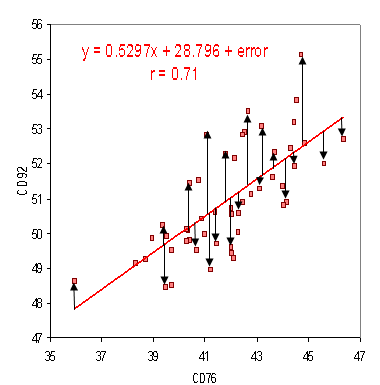
This function is then taken to be our “loss” function - a measure of how badly we are doing. In general we want to minimize this.

43.12.1.3.1. Optimization Problem#

The typical recipe for machine learning algorithms is to define a loss function of the parameters of a hypothesis, then to minimize the loss function. In our case we have the optimization problem

\[\min_{\mathbf{a}} \frac{1}{n} \sum_{i=1}^n (y^{(i)} - \mathbf{a}^\top\mathbf{X}^{(i)})^2\]

Note that we have added the bias into the design matrix.

43.12.1.3.2. Normal Equations#

Linear regression actually has a closed-form solution - the normal equation. It is beyond our scope to show the derivation, but here it is:

\[\mathbf{a}^* = (\mathbf{X}^\top\mathbf{X})^{-1}\mathbf{X}^\top \mathbf{y}\]

We won’t be implementing this equation, but you should know this is what sklearn.linear_model.LinearRegression is doing under the hood. We will talk more about optimization in later tutorials, where we have no closed-form solution.

43.12.1.4. Normalization#

It is generally a good idea to normalize all the values in the design matrix. This means all values should be in the range \((0, 1)\) and centered around zero.

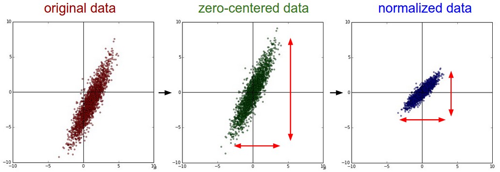
Normalization usually helps the learning algorithm perform better.

43.12.2. Example 1#

Simple Linear Regression

43.12.3. Importing the libraries#

%matplotlib inline
import numpy as np
import matplotlib.pyplot as plt
import pandas as pd

43.12.4. Importing the dataset#

dataset = pd.read_csv('../../assets/data/Salary_Data.csv')
X = dataset.iloc[:, :-1].values
y = dataset.iloc[:, -1].values

43.12.5. Splitting the dataset into the Training set and Test set#

from sklearn.model_selection import train_test_split

X_train, X_test, y_train, y_test = train_test_split(X, y, test_size = 1/3, random_state = 0)

43.12.6. Training the Simple Linear Regression model on the Training set#

from sklearn.linear_model import LinearRegression

regressor = LinearRegression()
regressor.fit(X_train, y_train)

43.12.7. Predicting the Test set results#

y_pred = regressor.predict(X_test)

43.12.8. Visualising the Training set results#

plt.scatter(X_train, y_train, color = 'red')
plt.plot(X_train, regressor.predict(X_train), color = 'blue')
plt.title('Salary vs Experience (Training set)')
plt.xlabel('Years of Experience')
plt.ylabel('Salary')
plt.show()

43.12.9. Visualising the Test set results#

plt.scatter(X_test, y_test, color = 'red')
plt.plot(X_train, regressor.predict(X_train), color = 'blue')
plt.title('Salary vs Experience (Test set)')
plt.xlabel('Years of Experience')
plt.ylabel('Salary')
plt.show()

43.12.10. Example 2#

Multiple Linear Regression

43.12.11. Importing the libraries#

%matplotlib inline
import numpy as np
import matplotlib.pyplot as plt
import pandas as pd

43.12.12. Importing the dataset#

dataset = pd.read_csv('../../assets/data/50_Startups.csv')
X = dataset.iloc[:, :-1].values
y = dataset.iloc[:, -1].values

print(X)

print(y)

43.12.13. Encoding categorical data#

from sklearn.compose import ColumnTransformer
from sklearn.preprocessing import OneHotEncoder
ct = ColumnTransformer(transformers=[('encoder', OneHotEncoder(), [3])], remainder='passthrough')
X = np.array(ct.fit_transform(X))

print(X)

43.12.14. Splitting the dataset into the Training set and Test set#

from sklearn.model_selection import train_test_split
X_train, X_test, y_train, y_test = train_test_split(X, y, test_size = 0.2, random_state = 0)

43.12.15. Training the Multiple Linear Regression model on the Training set#

from sklearn.linear_model import LinearRegression
regressor = LinearRegression()
regressor.fit(X_train, y_train)

43.12.16. Predicting the Test set results#

y_pred = regressor.predict(X_test)
np.set_printoptions(precision=2)
print(np.concatenate((y_pred.reshape(len(y_pred),1), y_test.reshape(len(y_test),1)),1))

43.12.17. Example 3#

Polynomial Linear Regression

43.12.18. Importing the libraries#

%matplotlib inline
import numpy as np
import matplotlib.pyplot as plt
import pandas as pd

43.12.19. Importing the dataset#

dataset = pd.read_csv('../../assets/data/Position_Salaries.csv')
X = dataset.iloc[:, 1:-1].values
y = dataset.iloc[:, -1].values

43.12.20. Training the Linear Regression model on the whole dataset#

from sklearn.linear_model import LinearRegression
lin_reg = LinearRegression()
lin_reg.fit(X, y)

43.12.21. Training the Polynomial Regression model on the whole dataset#

from sklearn.preprocessing import PolynomialFeatures
poly_transformer = PolynomialFeatures(degree = 4)
X_poly = poly_transformer.fit_transform(X)
lin_reg_2 = LinearRegression()
lin_reg_2.fit(X_poly, y)

43.12.22. Visualising the Polynomial Linear Regression results#

plt.scatter(X, y, color = 'red')
plt.plot(X, lin_reg.predict(X), color = 'blue')
plt.title('Truth or Bluff (Linear Regression)')
plt.xlabel('Position Level')
plt.ylabel('Salary')
plt.show()

43.12.23. Implementation of Linear Regression for scratch#

class MyOwnLinearRegression:
    def __init__(self, learning_rate=0.0001, n_iters=30000):
        self.lr = learning_rate
        self.n_iters = n_iters
        self.weights = None
        self.bias = None

    def fit(self, X, y):
        n_samples, n_features = X.shape

        # init parameters
        self.weights = np.zeros(n_features)
        self.bias = 0

        # gradient descent
        for _ in range(self.n_iters):
            # approximate y with linear combination of weights and x, plus bias
            y_predicted = np.dot(X, self.weights) + self.bias

            # compute gradients
            dw = (1 / n_samples) * np.dot(X.T, (y_predicted - y))
            db = (1 / n_samples) * np.sum(y_predicted - y)
            # update parameters
            self.weights  = self.weights - self.lr * dw
            self.bias  = self.bias -  self.lr * db

    def predict(self, X):
        y_predicted = np.dot(X, self.weights) + self.bias
        return y_predicted

43.12.24. Traning model with our own Linear Regression#

dataset = pd.read_csv('../../assets/data/Salary_Data.csv')
X = dataset.iloc[:, :-1].values
y = dataset.iloc[:, -1].values
X_train, X_test, y_train, y_test = train_test_split(X, y, test_size = 1/3, random_state = 0)
regressor = MyOwnLinearRegression()
regressor.fit(X_train, y_train)
y_pred = regressor.predict(X_test)

43.12.25. Visualising the Training set results#

plt.scatter(X_train, y_train, color = 'red')
plt.plot(X_train, regressor.predict(X_train), color = 'blue')
plt.title('Salary vs Experience (Training set)')
plt.xlabel('Years of Experience')
plt.ylabel('Salary')
plt.show()

43.12.26. Acknowledgments#

Thanks to TIM NIVEN for creating the open-source Kaggle jupyter notebook, licensed under Apache 2.0. It inspires the majority of the content of this assignment.

Ocademy Open Machine Learning Book

Linear Regression

Contents