42.66. Support Vector Machines (SVM) - Intro and SVM for Regression#

Support Vector Machines are the type of supervised learning algorithms used for regression, classification and detecting outliers. SVMs are remarkably one of the powerful models in classical machine learning suited for handling complex and high dimensional datasets.

With SVM supporting different kernels (linear, polynomial, Radial Basis Function(rbf), and sigmoid), SVM can tackle different kinds of datasets, both linear and non linear.

While the maths behind the SVMs are beyond the scope of this notebook, here is the idea behind SVMs:

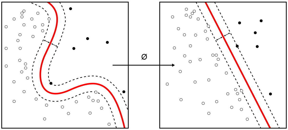
The way SVM works can be compared to a street with a boundary line. During SVM training, SMV draws the large margin or decision boundary between classes based on the importance of each training data point. The training data points that are inside the decision boundary are called support vectors and hence the name.

SVM

SMVs are widely used for classification. But to motivate that, let’s start with regression. For the purpose of examining how powerful this algorithm is, we will use the same dataset that we used in linear regression notebook, and hopefully the difference in performance will be notable.

42.66.2. 1 - Imports#

import numpy as np
import pandas as pd
import seaborn as sns
import urllib.request
import sklearn
import matplotlib.pyplot as plt
%matplotlib inline

42.66.3. 2 - Loading the data#

cal_data = pd.read_csv("../../assets/data/housing.csv")
cal_data.head()

	longitude	latitude	housing_median_age	total_rooms	total_bedrooms	population	households	median_income	median_house_value	ocean_proximity
0	-122.23	37.88	41.0	880.0	129.0	322.0	126.0	8.3252	452600.0	NEAR BAY
1	-122.22	37.86	21.0	7099.0	1106.0	2401.0	1138.0	8.3014	358500.0	NEAR BAY
2	-122.24	37.85	52.0	1467.0	190.0	496.0	177.0	7.2574	352100.0	NEAR BAY
3	-122.25	37.85	52.0	1274.0	235.0	558.0	219.0	5.6431	341300.0	NEAR BAY
4	-122.25	37.85	52.0	1627.0	280.0	565.0	259.0	3.8462	342200.0	NEAR BAY

len(cal_data)

42.66.4. 3 - Exploratory Analysis#

This is going to be a quick glance through the dataset. The full exploratory data analysis was done in the linear regression notebook[ADD LINK]. Before anything, let’s split the data into training and test set.

from sklearn.model_selection import train_test_split

train_data, test_data = train_test_split(cal_data, test_size=0.1,random_state=20)

print('The size of training data is: {} \nThe size of testing data is: {}'.format(len(train_data), len(test_data)))

The size of training data is: 18576 
The size of testing data is: 2064

## Checking statistics

train_data.describe().transpose()

	count	mean	std	min	25%	50%	75%	max
longitude	18576.0	-119.567530	2.000581	-124.3500	-121.7900	-118.4900	-118.010000	-114.4900
latitude	18576.0	35.630217	2.133260	32.5400	33.9300	34.2600	37.710000	41.9500
housing_median_age	18576.0	28.661068	12.604039	1.0000	18.0000	29.0000	37.000000	52.0000
total_rooms	18576.0	2631.567453	2169.467450	2.0000	1445.0000	2127.0000	3149.000000	39320.0000
total_bedrooms	18390.0	537.344698	417.672864	1.0000	295.0000	435.0000	648.000000	6445.0000
population	18576.0	1422.408376	1105.486111	3.0000	785.7500	1166.0000	1725.000000	28566.0000
households	18576.0	499.277078	379.473497	1.0000	279.0000	410.0000	606.000000	6082.0000
median_income	18576.0	3.870053	1.900225	0.4999	2.5643	3.5341	4.742725	15.0001
median_house_value	18576.0	206881.011305	115237.605962	14999.0000	120000.0000	179800.0000	264700.000000	500001.0000

## Checking missing values

train_data.isnull().sum()

longitude               0
latitude                0
housing_median_age      0
total_rooms             0
total_bedrooms        186
population              0
households              0
median_income           0
median_house_value      0
ocean_proximity         0
dtype: int64

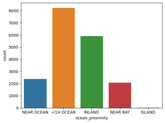
# Checking Values in the Categorical Feature(s)

train_data['ocean_proximity'].value_counts()

<1H OCEAN     8231
INLAND        5896
NEAR OCEAN    2384
NEAR BAY      2061
ISLAND           4
Name: ocean_proximity, dtype: int64

sns.countplot(data=train_data, x='ocean_proximity')

<AxesSubplot: xlabel='ocean_proximity', ylabel='count'>

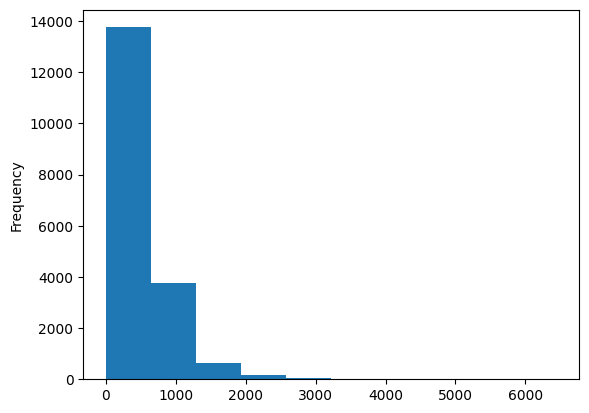
../../../_images/support_vector_machines_for_regression_13_1.png

Total bedroom is the only feature having missing values. Here is its distribution.

train_data['total_bedrooms'].plot(kind='hist')

<AxesSubplot: ylabel='Frequency'>

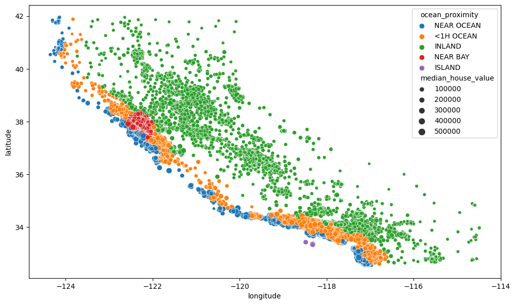
../../../_images/support_vector_machines_for_regression_15_1.png

# Plotting geographical features

plt.figure(figsize=(12,7))

sns.scatterplot(data = train_data, x='longitude', y='latitude', hue='ocean_proximity', 
                size='median_house_value')

<AxesSubplot: xlabel='longitude', ylabel='latitude'>

../../../_images/support_vector_machines_for_regression_16_1.png

42.66.5. 4 - Data Preprocessing#

To do:

Handle missing values
Encode categorical features
Scale the features
Everything into pipeline

# Getting training input data and labels

training_input_data = train_data.drop('median_house_value', axis=1)
training_labels = train_data['median_house_value']

# Numerical features 

num_feats = training_input_data.drop('ocean_proximity', axis=1)

# Categorical features 
cat_feats = training_input_data[['ocean_proximity']]

# Handle missing values 

from sklearn.pipeline import Pipeline 
from sklearn.impute import SimpleImputer
from sklearn.preprocessing import StandardScaler

num_pipe = Pipeline([
      ('imputer', SimpleImputer(strategy='mean')),
      ('scaler', StandardScaler())

    ])

num_preprocessed = num_pipe.fit_transform(num_feats)

# Pipeline to combine the numerical pipeline and also encode categorical features 
from sklearn.compose import ColumnTransformer
from sklearn.preprocessing import OneHotEncoder

# The transformer requires lists of features

num_list = list(num_feats)
cat_list = list(cat_feats)

final_pipe = ColumnTransformer([
    ('num', num_pipe, num_list),
    ('cat', OneHotEncoder(), cat_list)
])

training_data_preprocessed = final_pipe.fit_transform(training_input_data)

training_data_preprocessed

array([[ 0.67858615, -0.85796668,  0.97899282, ...,  0.        ,
         0.        ,  1.        ],
       [-0.93598814,  0.41242353,  0.18557502, ...,  0.        ,
         0.        ,  0.        ],
       [-1.45585107,  0.9187045 ,  0.02689146, ...,  0.        ,
         0.        ,  1.        ],
       ...,
       [ 1.27342931, -1.32674535,  0.18557502, ...,  0.        ,
         0.        ,  0.        ],
       [ 0.64859406, -0.71733307,  0.97899282, ...,  0.        ,
         0.        ,  0.        ],
       [-1.44085502,  1.01246024,  1.37570172, ...,  0.        ,
         1.        ,  0.        ]])

42.66.6. 5 - Training Support Vector Regressor#

In regression, instead of separating the classes with decision boundary like in classification, SVR fits the training data points on the boundary margin but keep them off.

We can implement it quite easily with Scikit-Learn.

from sklearn.svm import LinearSVR, SVR

lin_svr = LinearSVR()
lin_svr.fit(training_data_preprocessed, training_labels)

LinearSVR()

In a Jupyter environment, please rerun this cell to show the HTML representation or trust the notebook.
On GitHub, the HTML representation is unable to render, please try loading this page with nbviewer.org.

We can also use nonlinear SVM with a polynomial kernel function.

poly_svr = SVR(kernel='poly')
poly_svr.fit(training_data_preprocessed, training_labels)

SVR(kernel='poly')

42.66.7. 6 - Evaluating Support Vector Regressor#

Let us evaluate the two models we created on the training set before evaluating on the test set. This is a good practice. Since finding a good model can take many iterations of improvements, it’s not advised to touch the test set until the model is good enough. Otherwise it would fail to make predictions on the new data.

As always, we evaluate regression models with mean squarred error, but the commonly used one is root mean squarred error.

from sklearn.metrics import mean_squared_error

predictions = lin_svr.predict(training_data_preprocessed)
mse = mean_squared_error(training_labels, predictions)
rmse = np.sqrt(mse)
rmse

215682.86713461558

That’s too high error. Let’s see how SVR with polynomial kernel will perform.

predictions = poly_svr.predict(training_data_preprocessed)
mse = mean_squared_error(training_labels, predictions)
rmse = np.sqrt(mse)
rmse

117513.38828582528

It did well than the former. For now, we can try to improve this with Randomized Search where we can find the best parameters. Let’s do that!

42.66.8. 7 - Improving Support Vector Regressor#

Let use Randomized Search to improve the SVR model. Few notes about the parameters:

Gamma(y): This is a regularization hyperparameter. When gamma is small, the model can underfit. It is too high, model can overfit.
C: It’s same as gamma. It is a regularization hyperparameter. When C is low, there is much regularization. When C is high, there is low regularization.
epsilon: is used to control the width of the street.

from sklearn.model_selection import RandomizedSearchCV

params = {'gamma':[0.0001, 0.1],'C':[1,1000], 'epsilon':[0,0.5], 'degree':[2,5]}

rnd_search = RandomizedSearchCV(SVR(), params, n_iter=10, verbose=2, cv=3, random_state=42)

rnd_search.fit(training_data_preprocessed, training_labels)

Fitting 3 folds for each of 10 candidates, totalling 30 fits
[CV] END .............C=1, degree=2, epsilon=0, gamma=0.0001; total time=  17.0s
[CV] END .............C=1, degree=2, epsilon=0, gamma=0.0001; total time=  16.2s
[CV] END .............C=1, degree=2, epsilon=0, gamma=0.0001; total time=  15.4s
[CV] END ................C=1, degree=2, epsilon=0, gamma=0.1; total time=  15.1s
[CV] END ................C=1, degree=2, epsilon=0, gamma=0.1; total time=  15.2s
[CV] END ................C=1, degree=2, epsilon=0, gamma=0.1; total time=  15.1s
[CV] END ................C=1, degree=5, epsilon=0, gamma=0.1; total time=  15.4s
[CV] END ................C=1, degree=5, epsilon=0, gamma=0.1; total time=  16.7s
[CV] END ................C=1, degree=5, epsilon=0, gamma=0.1; total time=  14.8s
[CV] END ........C=1000, degree=5, epsilon=0.5, gamma=0.0001; total time=  15.1s
[CV] END ........C=1000, degree=5, epsilon=0.5, gamma=0.0001; total time=  15.3s
[CV] END ........C=1000, degree=5, epsilon=0.5, gamma=0.0001; total time=  16.9s
[CV] END .............C=1000, degree=5, epsilon=0, gamma=0.1; total time=  17.8s
[CV] END .............C=1000, degree=5, epsilon=0, gamma=0.1; total time=  20.4s
[CV] END .............C=1000, degree=5, epsilon=0, gamma=0.1; total time=  18.1s
[CV] END ...........C=1000, degree=2, epsilon=0.5, gamma=0.1; total time=  20.8s
[CV] END ...........C=1000, degree=2, epsilon=0.5, gamma=0.1; total time=  23.3s
[CV] END ...........C=1000, degree=2, epsilon=0.5, gamma=0.1; total time=  22.2s
[CV] END ..........C=1000, degree=2, epsilon=0, gamma=0.0001; total time=  20.6s
[CV] END ..........C=1000, degree=2, epsilon=0, gamma=0.0001; total time=  20.1s
[CV] END ..........C=1000, degree=2, epsilon=0, gamma=0.0001; total time=  20.3s
[CV] END .............C=1000, degree=2, epsilon=0, gamma=0.1; total time=  19.0s
[CV] END .............C=1000, degree=2, epsilon=0, gamma=0.1; total time=  18.9s
[CV] END .............C=1000, degree=2, epsilon=0, gamma=0.1; total time=  19.7s
[CV] END ...........C=1, degree=2, epsilon=0.5, gamma=0.0001; total time=  23.5s
[CV] END ...........C=1, degree=2, epsilon=0.5, gamma=0.0001; total time=  27.7s
[CV] END ...........C=1, degree=2, epsilon=0.5, gamma=0.0001; total time=  17.9s
[CV] END ...........C=1000, degree=5, epsilon=0.5, gamma=0.1; total time=  16.7s
[CV] END ...........C=1000, degree=5, epsilon=0.5, gamma=0.1; total time=  16.7s
[CV] END ...........C=1000, degree=5, epsilon=0.5, gamma=0.1; total time=  15.2s

RandomizedSearchCV(cv=3, estimator=SVR(),
                   param_distributions={'C': [1, 1000], 'degree': [2, 5],
                                        'epsilon': [0, 0.5],
                                        'gamma': [0.0001, 0.1]},
                   random_state=42, verbose=2)

We can now find the best parameters

rnd_search.best_params_

{'gamma': 0.1, 'epsilon': 0, 'degree': 5, 'C': 1000}

svr_rnd = rnd_search.best_estimator_.fit(training_data_preprocessed, training_labels)

Now, let’s evaluate it on the training set

predictions = svr_rnd.predict(training_data_preprocessed)
mse = mean_squared_error(training_labels, predictions)
rmse = np.sqrt(mse)
rmse

68684.15262765526

Wow, this is much bettter. We were able to improve reduce the root mean squarred error from $117,513 to $68,684.

Now, we can evaluate the model on the test set. We will have to transform it the same way we transformed the training set for the prediction to be possible.

test_input_data = test_data.drop('median_house_value', axis=1)
test_labels = test_data['median_house_value']


test_preprocessed = final_pipe.transform(test_input_data)

test_pred = svr_rnd.predict(test_preprocessed)
test_mse = mean_squared_error(test_labels,test_pred)

test_rmse = np.sqrt(test_mse)
test_rmse

68478.07737338323

That’s is not really bad.

This is the end of the notebook. It was a practical introduction to using Support Vector Machines for regression. In the next lab, we will take a further step, where we will do classification with SVM.

42.66.9. Acknowledgments#

Thanks to Jake VanderPlas for creating the open-source course Python Data Science Handbook . It inspires the majority of the content in this chapter.

Ocademy Open Machine Learning Book

Support Vector Machines (SVM) - Intro and SVM for Regression

Contents