Word embedding
Contents
# Install the necessary dependencies

import os
import sys
!{sys.executable} -m pip install --quiet pandas scikit-learn numpy matplotlib jupyterlab_myst ipython gensim torch
30.7.2. Word embedding#
Word Embeddings are numeric representations of words in a lower-dimensional space, capturing semantic and syntactic information. Mainly including discrete representation methods and distribution representation methods
30.7.2.1. Discrete representation#
This method involves compiling a list of distinct terms and giving each one a unique integer value, or id. and after that, insert each word’s distinct id into the sentence. Every vocabulary word is handled as a feature in this instance. Thus, a large vocabulary will result in an extremely large feature size. Common discrete representation methods include:one-hot,Bag of Word (Bow) and Term frequency-inverse document frequency (TF-IDF)
30.7.2.1.1. One-Hot#
One-hot encoding is a simple method for representing words in natural language processing (NLP). In this encoding scheme, each word in the vocabulary is represented as a unique vector, where the dimensionality of the vector is equal to the size of the vocabulary. The vector has all elements set to 0, except for the element corresponding to the index of the word in the vocabulary, which is set to 1.
def one_hot_encode(text):
	words = text.split()
	vocabulary = set(words)
	word_to_index = {word: i for i, word in enumerate(vocabulary)}
	one_hot_encoded = []
	for word in words:
		one_hot_vector = [0] * len(vocabulary)
		one_hot_vector[word_to_index[word]] = 1
		one_hot_encoded.append(one_hot_vector)

	return one_hot_encoded, word_to_index, vocabulary

# sample
example_text = "cat in the hat dog on the mat bird in the tree"

one_hot_encoded, word_to_index, vocabulary = one_hot_encode(example_text)

print("Vocabulary:", vocabulary)
print("Word to Index Mapping:", word_to_index)
print("One-Hot Encoded Matrix:")
for word, encoding in zip(example_text.split(), one_hot_encoded):
	print(f"{word}: {encoding}")
Vocabulary: {'mat', 'dog', 'tree', 'in', 'on', 'hat', 'the', 'bird', 'cat'}
Word to Index Mapping: {'mat': 0, 'dog': 1, 'tree': 2, 'in': 3, 'on': 4, 'hat': 5, 'the': 6, 'bird': 7, 'cat': 8}
One-Hot Encoded Matrix:
cat: [0, 0, 0, 0, 0, 0, 0, 0, 1]
in: [0, 0, 0, 1, 0, 0, 0, 0, 0]
the: [0, 0, 0, 0, 0, 0, 1, 0, 0]
hat: [0, 0, 0, 0, 0, 1, 0, 0, 0]
dog: [0, 1, 0, 0, 0, 0, 0, 0, 0]
on: [0, 0, 0, 0, 1, 0, 0, 0, 0]
the: [0, 0, 0, 0, 0, 0, 1, 0, 0]
mat: [1, 0, 0, 0, 0, 0, 0, 0, 0]
bird: [0, 0, 0, 0, 0, 0, 0, 1, 0]
in: [0, 0, 0, 1, 0, 0, 0, 0, 0]
the: [0, 0, 0, 0, 0, 0, 1, 0, 0]
tree: [0, 0, 1, 0, 0, 0, 0, 0, 0]
30.7.2.1.2. Bag of Word (Bow)#
Bag-of-Words (BoW) is a text representation technique that represents a document as an unordered set of words and their respective frequencies. It discards the word order and captures the frequency of each word in the document, creating a vector representation.
from sklearn.feature_extraction.text import CountVectorizer
documents = ["This is the first document.",
			"This document is the second document.",
			"And this is the third one.",
			"Is this the first document?"]

vectorizer = CountVectorizer()
X = vectorizer.fit_transform(documents)
feature_names = vectorizer.get_feature_names_out()

print("Bag-of-Words Matrix:")
print(X.toarray())
print("Vocabulary (Feature Names):", feature_names)
Bag-of-Words Matrix:
[[0 1 1 1 0 0 1 0 1]
 [0 2 0 1 0 1 1 0 1]
 [1 0 0 1 1 0 1 1 1]
 [0 1 1 1 0 0 1 0 1]]
Vocabulary (Feature Names): ['and' 'document' 'first' 'is' 'one' 'second' 'the' 'third' 'this']
30.7.2.1.3. Term frequency-inverse document frequency (TF-IDF)#
Term Frequency-Inverse Document Frequency, commonly known as TF-IDF, is a numerical statistic that reflects the importance of a word in a document relative to a collection of documents (corpus). It is widely used in natural language processing and information retrieval to evaluate the significance of a term within a specific document in a larger corpus. TF-IDF consists of two components:
·Term Frequency (TF): Term Frequency measures how often a term (word) appears in a document. It is calculated using the formula:
\(TF(t,d)=\frac{Total\ number\ of\ times\ term\ t\ appears\ in\ document\ d}{Total\ number\ of\ terms\ in\ document\ d}\)
·Inverse Document Frequency (IDF): Inverse Document Frequency measures the importance of a term across a collection of documents. It is calculated using the formula:
\(IDF(t,D)=\log{(\frac{Total\ documents}{Number\ of\ documents\ containing\ term\ t})}\)
The TF-IDF score for a term t in a document d is then given by multiplying the TF and IDF values:
TF-IDF(t,d,D)=TF(t,d)×IDF(t,D)
The higher the TF-IDF score for a term in a document, the more important that term is to that document within the context of the entire corpus. This weighting scheme helps in identifying and extracting relevant information from a large collection of documents, and it is commonly used in text mining, information retrieval, and document clustering.
Let’s Implement Term Frequency-Inverse Document Frequency (TF-IDF) using python with the scikit-learn library. It begins by defining a set of sample documents. The TfidfVectorizer is employed to transform these documents into a TF-IDF matrix. The code then extracts and prints the TF-IDF values for each word in each document. This statistical measure helps assess the importance of words in a document relative to their frequency across a collection of documents, aiding in information retrieval and text analysis tasks.
from sklearn.feature_extraction.text import TfidfVectorizer

# Sample
documents = [
	"The quick brown fox jumps over the lazy dog.",
	"A journey of a thousand miles begins with a single step.",
]

vectorizer = TfidfVectorizer() # Create the TF-IDF vectorizer
tfidf_matrix = vectorizer.fit_transform(documents)
feature_names = vectorizer.get_feature_names_out()
tfidf_values = {}

for doc_index, doc in enumerate(documents):
	feature_index = tfidf_matrix[doc_index, :].nonzero()[1]
	tfidf_doc_values = zip(feature_index, [tfidf_matrix[doc_index, x] for x in feature_index])
	tfidf_values[doc_index] = {feature_names[i]: value for i, value in tfidf_doc_values}
#let's print
for doc_index, values in tfidf_values.items():
	print(f"Document {doc_index + 1}:")
	for word, tfidf_value in values.items():
		print(f"{word}: {tfidf_value}")
	print("\n")
Document 1:
dog: 0.30151134457776363
lazy: 0.30151134457776363
over: 0.30151134457776363
jumps: 0.30151134457776363
fox: 0.30151134457776363
brown: 0.30151134457776363
quick: 0.30151134457776363
the: 0.6030226891555273


Document 2:
step: 0.3535533905932738
single: 0.3535533905932738
with: 0.3535533905932738
begins: 0.3535533905932738
miles: 0.3535533905932738
thousand: 0.3535533905932738
of: 0.3535533905932738
journey: 0.3535533905932738
30.7.2.2. Distributed representation#
30.7.2.2.1. Word2Vec#
Word2Vec is a neural approach for generating word embeddings. It belongs to the family of neural word embedding techniques and specifically falls under the category of distributed representation models. It is a popular technique in natural language processing (NLP) that is used to represent words as continuous vector spaces. Developed by a team at Google, Word2Vec aims to capture the semantic relationships between words by mapping them to high-dimensional vectors. The underlying idea is that words with similar meanings should have similar vector representations. In Word2Vec every word is assigned a vector. We start with either a random vector or one-hot vector.
There are two neural embedding methods for Word2Vec, Continuous Bag of Words (CBOW) and Skip-gram.
30.7.2.2.1.1. Continuous Bag of Words(CBOW)#
Continuous Bag of Words (CBOW) is a type of neural network architecture used in the Word2Vec model. The primary objective of CBOW is to predict a target word based on its context, which consists of the surrounding words in a given window. Given a sequence of words in a context window, the model is trained to predict the target word at the center of the window.
CBOW is a feedforward neural network with a single hidden layer. The input layer represents the context words, and the output layer represents the target word. The hidden layer contains the learned continuous vector representations (word embeddings) of the input words.
The architecture is useful for learning distributed representations of words in a continuous vector space.
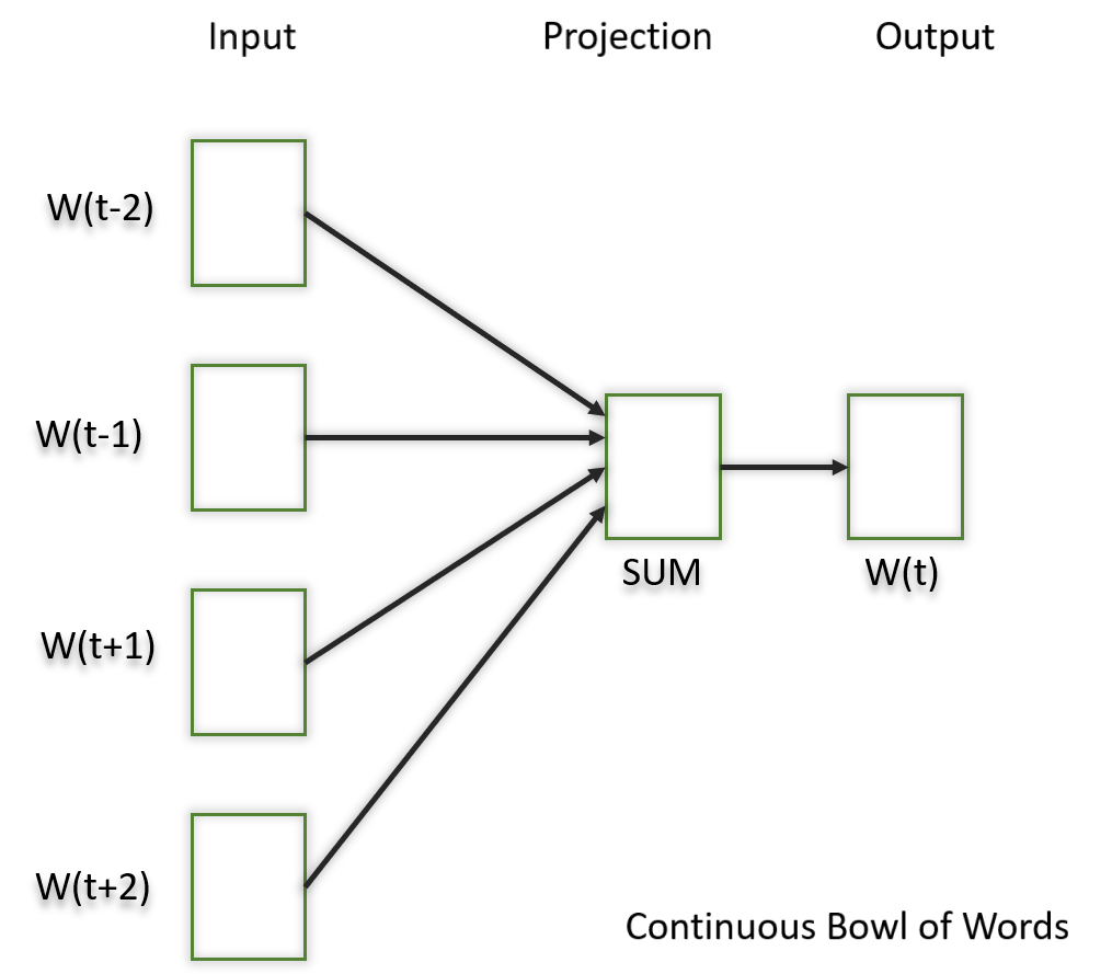
Fig. 30.6 Continuous Bag of Words#
The hidden layer contains the continuous vector representations (word embeddings) of the input words.
The weights between the input layer and the hidden layer are learned during training. The dimensionality of the hidden layer represents the size of the word embeddings (the continuous vector space).
import torch
import torch.nn as nn
import torch.optim as optim

# Define CBOW model
class CBOWModel(nn.Module):
	def __init__(self, vocab_size, embed_size):
		super(CBOWModel, self).__init__()
		self.embeddings = nn.Embedding(vocab_size, embed_size)
		self.linear = nn.Linear(embed_size, vocab_size)

	def forward(self, context):
		context_embeds = self.embeddings(context).sum(dim=1)
		output = self.linear(context_embeds)
		return output

# Sample data
context_size = 2
raw_text = "word embeddings are awesome"
tokens = raw_text.split()
vocab = set(tokens)
word_to_index = {word: i for i, word in enumerate(vocab)}
data = []
for i in range(2, len(tokens) - 2):
	context = [word_to_index[word] for word in tokens[i - 2:i] + tokens[i + 1:i + 3]]
	target = word_to_index[tokens[i]]
	data.append((torch.tensor(context), torch.tensor(target)))

# Hyperparameters
vocab_size = len(vocab)
embed_size = 10
learning_rate = 0.01
epochs = 100

# Initialize CBOW model
cbow_model = CBOWModel(vocab_size, embed_size)
criterion = nn.CrossEntropyLoss()
optimizer = optim.SGD(cbow_model.parameters(), lr=learning_rate)

# Training loop
for epoch in range(epochs):
	total_loss = 0
	for context, target in data:
		optimizer.zero_grad()
		output = cbow_model(context)
		loss = criterion(output.unsqueeze(0), target.unsqueeze(0))
		loss.backward()
		optimizer.step()
		total_loss += loss.item()
	print(f"Epoch {epoch + 1}, Loss: {total_loss}")

# Example usage: Get embedding for a specific word
word_to_lookup = "embeddings"
word_index = word_to_index[word_to_lookup]
embedding = cbow_model.embeddings(torch.tensor([word_index]))
print(f"Embedding for '{word_to_lookup}': {embedding.detach().numpy()}")
Epoch 1, Loss: 0
Epoch 2, Loss: 0
Epoch 3, Loss: 0
Epoch 4, Loss: 0
Epoch 5, Loss: 0
Epoch 6, Loss: 0
Epoch 7, Loss: 0
Epoch 8, Loss: 0
Epoch 9, Loss: 0
Epoch 10, Loss: 0
Epoch 11, Loss: 0
Epoch 12, Loss: 0
Epoch 13, Loss: 0
Epoch 14, Loss: 0
Epoch 15, Loss: 0
Epoch 16, Loss: 0
Epoch 17, Loss: 0
Epoch 18, Loss: 0
Epoch 19, Loss: 0
Epoch 20, Loss: 0
Epoch 21, Loss: 0
Epoch 22, Loss: 0
Epoch 23, Loss: 0
Epoch 24, Loss: 0
Epoch 25, Loss: 0
Epoch 26, Loss: 0
Epoch 27, Loss: 0
Epoch 28, Loss: 0
Epoch 29, Loss: 0
Epoch 30, Loss: 0
Epoch 31, Loss: 0
Epoch 32, Loss: 0
Epoch 33, Loss: 0
Epoch 34, Loss: 0
Epoch 35, Loss: 0
Epoch 36, Loss: 0
Epoch 37, Loss: 0
Epoch 38, Loss: 0
Epoch 39, Loss: 0
Epoch 40, Loss: 0
Epoch 41, Loss: 0
Epoch 42, Loss: 0
Epoch 43, Loss: 0
Epoch 44, Loss: 0
Epoch 45, Loss: 0
Epoch 46, Loss: 0
Epoch 47, Loss: 0
Epoch 48, Loss: 0
Epoch 49, Loss: 0
Epoch 50, Loss: 0
Epoch 51, Loss: 0
Epoch 52, Loss: 0
Epoch 53, Loss: 0
Epoch 54, Loss: 0
Epoch 55, Loss: 0
Epoch 56, Loss: 0
Epoch 57, Loss: 0
Epoch 58, Loss: 0
Epoch 59, Loss: 0
Epoch 60, Loss: 0
Epoch 61, Loss: 0
Epoch 62, Loss: 0
Epoch 63, Loss: 0
Epoch 64, Loss: 0
Epoch 65, Loss: 0
Epoch 66, Loss: 0
Epoch 67, Loss: 0
Epoch 68, Loss: 0
Epoch 69, Loss: 0
Epoch 70, Loss: 0
Epoch 71, Loss: 0
Epoch 72, Loss: 0
Epoch 73, Loss: 0
Epoch 74, Loss: 0
Epoch 75, Loss: 0
Epoch 76, Loss: 0
Epoch 77, Loss: 0
Epoch 78, Loss: 0
Epoch 79, Loss: 0
Epoch 80, Loss: 0
Epoch 81, Loss: 0
Epoch 82, Loss: 0
Epoch 83, Loss: 0
Epoch 84, Loss: 0
Epoch 85, Loss: 0
Epoch 86, Loss: 0
Epoch 87, Loss: 0
Epoch 88, Loss: 0
Epoch 89, Loss: 0
Epoch 90, Loss: 0
Epoch 91, Loss: 0
Epoch 92, Loss: 0
Epoch 93, Loss: 0
Epoch 94, Loss: 0
Epoch 95, Loss: 0
Epoch 96, Loss: 0
Epoch 97, Loss: 0
Epoch 98, Loss: 0
Epoch 99, Loss: 0
Epoch 100, Loss: 0
Embedding for 'embeddings': [[-1.0344244   0.07897425  0.03608504 -0.556515    0.14206451 -1.833232
   0.7083351   0.66258     0.57552516  1.7009653 ]]
30.7.2.2.1.2. Skip-Gram#
The Skip-Gram model learns distributed representations of words in a continuous vector space. The main objective of Skip-Gram is to predict context words (words surrounding a target word) given a target word. This is the opposite of the Continuous Bag of Words (CBOW) model, where the objective is to predict the target word based on its context. It is shown that this method produces more meaningful embeddings.

Fig. 30.7 Skip Gram#
After applying the above neural embedding methods we get trained vectors of each word after many iterations through the corpus. These trained vectors preserve syntactical or semantic information and are converted to lower dimensions. The vectors with similar meaning or semantic information are placed close to each other in space.
Let’s understand with a basic example. The python code contains, parameter that controls the dimensionality of the word vectors, and you can adjust other parameters such as based on your specific needs.vector_sizewindow
Note: Word2Vec models can perform better with larger datasets. If you have a large corpus, you might achieve more meaningful word embeddings.
!pip install gensim
from gensim.models import Word2Vec
from nltk.tokenize import word_tokenize
import nltk
nltk.download('punkt') # Download the tokenizer models if not already downloaded

sample = "Word embeddings are dense vector representations of words."
tokenized_corpus = word_tokenize(sample.lower()) # Lowercasing for consistency

skipgram_model = Word2Vec(sentences=[tokenized_corpus],
						vector_size=100, # Dimensionality of the word vectors
						window=5,		 # Maximum distance between the current and predicted word within a sentence
						sg=1,			 # Skip-Gram model (1 for Skip-Gram, 0 for CBOW)
						min_count=1,	 # Ignores all words with a total frequency lower than this
						workers=4)	 # Number of CPU cores to use for training the model

# Training
skipgram_model.train([tokenized_corpus], total_examples=1, epochs=10)
skipgram_model.save("skipgram_model.model")
loaded_model = Word2Vec.load("skipgram_model.model")
vector_representation = loaded_model.wv['word']
print("Vector representation of 'word':", vector_representation)
Requirement already satisfied: gensim in d:\anaconda\lib\site-packages (4.3.0)
Requirement already satisfied: FuzzyTM>=0.4.0 in d:\anaconda\lib\site-packages (from gensim) (2.0.5)
Requirement already satisfied: numpy>=1.18.5 in d:\anaconda\lib\site-packages (from gensim) (1.23.5)
Requirement already satisfied: scipy>=1.7.0 in d:\anaconda\lib\site-packages (from gensim) (1.10.0)
Requirement already satisfied: smart-open>=1.8.1 in d:\anaconda\lib\site-packages (from gensim) (5.2.1)
Requirement already satisfied: pyfume in d:\anaconda\lib\site-packages (from FuzzyTM>=0.4.0->gensim) (0.2.25)
Requirement already satisfied: pandas in d:\anaconda\lib\site-packages (from FuzzyTM>=0.4.0->gensim) (1.5.3)
Requirement already satisfied: python-dateutil>=2.8.1 in d:\anaconda\lib\site-packages (from pandas->FuzzyTM>=0.4.0->gensim) (2.8.2)
Requirement already satisfied: pytz>=2020.1 in d:\anaconda\lib\site-packages (from pandas->FuzzyTM>=0.4.0->gensim) (2022.7)
Requirement already satisfied: fst-pso in d:\anaconda\lib\site-packages (from pyfume->FuzzyTM>=0.4.0->gensim) (1.8.1)
Requirement already satisfied: simpful in d:\anaconda\lib\site-packages (from pyfume->FuzzyTM>=0.4.0->gensim) (2.11.0)
Requirement already satisfied: six>=1.5 in d:\anaconda\lib\site-packages (from python-dateutil>=2.8.1->pandas->FuzzyTM>=0.4.0->gensim) (1.16.0)
Requirement already satisfied: miniful in d:\anaconda\lib\site-packages (from fst-pso->pyfume->FuzzyTM>=0.4.0->gensim) (0.0.6)
[nltk_data] Downloading package punkt to
[nltk_data]     C:\Users\zhongmeiqi\AppData\Roaming\nltk_data...
[nltk_data]   Package punkt is already up-to-date!
Vector representation of 'word': [-9.5800208e-03  8.9437785e-03  4.1664648e-03  9.2367809e-03
  6.6457358e-03  2.9233587e-03  9.8055992e-03 -4.4231843e-03
 -6.8048164e-03  4.2256550e-03  3.7299085e-03 -5.6668529e-03
  9.7035142e-03 -3.5551414e-03  9.5499391e-03  8.3657773e-04
 -6.3355025e-03 -1.9741615e-03 -7.3781307e-03 -2.9811086e-03
  1.0425397e-03  9.4814906e-03  9.3598543e-03 -6.5986011e-03
  3.4773252e-03  2.2767992e-03 -2.4910474e-03 -9.2290826e-03
  1.0267317e-03 -8.1645092e-03  6.3240929e-03 -5.8001447e-03
  5.5353874e-03  9.8330071e-03 -1.5987856e-04  4.5296676e-03
 -1.8086446e-03  7.3613892e-03  3.9419360e-03 -9.0095028e-03
 -2.3953868e-03  3.6261671e-03 -1.0080514e-04 -1.2024897e-03
 -1.0558038e-03 -1.6681013e-03  6.0541567e-04  4.1633579e-03
 -4.2531900e-03 -3.8336846e-03 -5.0755290e-05  2.6549282e-04
 -1.7014991e-04 -4.7843382e-03  4.3120929e-03 -2.1710952e-03
  2.1056964e-03  6.6702347e-04  5.9686624e-03 -6.8418151e-03
 -6.8183104e-03 -4.4762432e-03  9.4359247e-03 -1.5930856e-03
 -9.4291316e-03 -5.4270827e-04 -4.4478951e-03  5.9980620e-03
 -9.5831212e-03  2.8602476e-03 -9.2544509e-03  1.2484600e-03
  6.0004774e-03  7.4001122e-03 -7.6209377e-03 -6.0561695e-03
 -6.8399287e-03 -7.9184016e-03 -9.4984965e-03 -2.1255787e-03
 -8.3757477e-04 -7.2564054e-03  6.7876028e-03  1.1183097e-03
  5.8291717e-03  1.4714618e-03  7.9081533e-04 -7.3718326e-03
 -2.1769912e-03  4.3199472e-03 -5.0856168e-03  1.1304744e-03
  2.8835384e-03 -1.5386029e-03  9.9318363e-03  8.3507905e-03
  2.4184163e-03  7.1170190e-03  5.8888551e-03 -5.5787875e-03]
In practice, the choice between CBOW and Skip-gram often depends on the specific characteristics of the data and the task at hand. CBOW might be preferred when training resources are limited, and capturing syntactic information is important. Skip-gram, on the other hand, might be chosen when semantic relationships and the representation of rare words are crucial.
30.7.2.3. Pretrained Word-Embedding#
Pre-trained word embeddings are representations of words that are learned from large corpora and are made available for reuse in various natural language processing (NLP) tasks. These embeddings capture semantic relationships between words, allowing the model to understand similarities and relationships between different words in a meaningful way.
30.7.2.3.1. GloVe#
GloVe is trained on global word co-occurrence statistics. It leverages the global context to create word embeddings that reflect the overall meaning of words based on their co-occurrence probabilities. this method, we take the corpus and iterate through it and get the co-occurrence of each word with other words in the corpus. We get a co-occurrence matrix through this. The words which occur next to each other get a value of 1, if they are one word apart then 1/2, if two words apart then 1/3 and so on.
Let us take an example to understand how the matrix is created. We have a small corpus:
Corpus:
It is a nice evening.
Good Evening!
Is it a nice evening?
it |
is |
a |
nice |
evening |
good |
|
|---|---|---|---|---|---|---|
it |
0 |
|||||
is |
1+1 |
0 |
||||
a |
1/2+1 |
1+1/2 |
0 |
|||
nice |
1/3+1/2 |
1/2+1/3 |
1+1 |
0 |
||
evening |
1/4+1/3 |
1/3+1/4 |
1/2+1/2 |
1+1 |
0 |
|
good |
0 |
0 |
0 |
0 |
1 |
0 |
The upper half of the matrix will be a reflection of the lower half. We can consider a window frame as well to calculate the co-occurrences by shifting the frame till the end of the corpus. This helps gather information about the context in which the word is used.
Initially, the vectors for each word is assigned randomly. Then we take two pairs of vectors and see how close they are to each other in space. If they occur together more often or have a higher value in the co-occurrence matrix and are far apart in space then they are brought close to each other. If they are close to each other but are rarely or not frequently used together then they are moved further apart in space.
After many iterations of the above process, we’ll get a vector space representation that approximates the information from the co-occurrence matrix. The performance of GloVe is better than Word2Vec in terms of both semantic and syntactic capturing.
from gensim.models import KeyedVectors
from gensim.downloader import load

glove_model = load('glove-wiki-gigaword-50')
word_pairs = [('learn', 'learning'), ('india', 'indian'), ('fame', 'famous')]

# Compute similarity for each pair of words
for pair in word_pairs:
	similarity = glove_model.similarity(pair[0], pair[1])
	print(f"Similarity between '{pair[0]}' and '{pair[1]}' using GloVe: {similarity:.3f}")
Output:
Similarity between ‘learn’ and ‘learning’ using GloVe: 0.802
Similarity between ‘india’ and ‘indian’ using GloVe: 0.865
Similarity between ‘fame’ and ‘famous’ using GloVe: 0.589
30.7.2.3.2. Fasttext#
Developed by Facebook, FastText extends Word2Vec by representing words as bags of character n-grams. This approach is particularly useful for handling out-of-vocabulary words and capturing morphological variations.
import gensim.downloader as api
fasttext_model = api.load("fasttext-wiki-news-subwords-300") ## Load the pre-trained fastText model
# Define word pairs to compute similarity for
word_pairs = [('learn', 'learning'), ('india', 'indian'), ('fame', 'famous')]

# Compute similarity for each pair of words
for pair in word_pairs:
	similarity = fasttext_model.similarity(pair[0], pair[1])
	print(f"Similarity between '{pair[0]}' and '{pair[1]}' using FastText: {similarity:.3f}")
Output:
Similarity between ‘learn’ and ‘learning’ using Word2Vec: 0.642
Similarity between ‘india’ and ‘indian’ using Word2Vec: 0.708
Similarity between ‘fame’ and ‘famous’ using Word2Vec: 0.519
30.7.2.3.3. BERT (Bidirectional Encoder Representations from Transformers)#
BERT is a transformer-based model that learns contextualized embeddings for words. It considers the entire context of a word by considering both left and right contexts, resulting in embeddings that capture rich contextual information.
from transformers import BertTokenizer, BertModel
import torch

# Load pre-trained BERT model and tokenizer
model_name = 'bert-base-uncased'
tokenizer = BertTokenizer.from_pretrained(model_name)
model = BertModel.from_pretrained(model_name)

word_pairs = [('learn', 'learning'), ('india', 'indian'), ('fame', 'famous')]

# Compute similarity for each pair of words
for pair in word_pairs:
	tokens = tokenizer(pair, return_tensors='pt')
	with torch.no_grad():
		outputs = model(**tokens)

	# Extract embeddings for the [CLS] token
	cls_embedding = outputs.last_hidden_state[:, 0, :]

	similarity = torch.nn.functional.cosine_similarity(cls_embedding[0], cls_embedding[1], dim=0)

	print(f"Similarity between '{pair[0]}' and '{pair[1]}' using BERT: {similarity:.3f}")
Output:
Similarity between ‘learn’ and ‘learning’ using BERT: 0.930
Similarity between ‘india’ and ‘indian’ using BERT: 0.957
Similarity between ‘fame’ and ‘famous’ using BERT: 0.956
30.7.2.4. Considerations for Deploying Word Embedding Models#
You need to use the exact same pipeline during deploying your model as were used to create the training data for the word embedding. If you use a different tokenizer or different method of handling white space, punctuation etc. you might end up with incompatible inputs.
Words in your input that doesn’t have a pre-trained vector. Such words are known as Out of Vocabulary Word(oov). What you can do is replace those words with “UNK” which means unknown and then handle them separately.
Dimension mis-match: Vectors can be of many lengths. If you train a model with vectors of length say 400 and then try to apply vectors of length 1000 at inference time, you will run into errors. So make sure to use the same dimensions throughout.
30.7.2.5. Advantages and Disadvantage of Word Embeddings#
30.7.2.5.1. Advantages#
It is much faster to train than hand build models like WordNet (which uses graph embeddings).
Almost all modern NLP applications start with an embedding layer.
It Stores an approximation of meaning.
30.7.2.5.2. Disadvantages#
It can be memory intensive.
It is corpus dependent. Any underlying bias will have an effect on your model.
It cannot distinguish between homophones. Eg: brake/break, cell/sell, weather/whether etc.
30.7.2.6. Conclusion#
In conclusion, word embedding techniques such as TF-IDF, Word2Vec, and GloVe play a crucial role in natural language processing by representing words in a lower-dimensional space, capturing semantic and syntactic information.
30.7.2.7. Your turn! 🚀#
Assignment - News topic classification tasks
30.7.2.8. Acknowledgments#
Thanks to GeeksforGeeks for creating the open-source project Word Embeddings in NLP.It inspire the majority of the content in this chapter.