42.74. Regularized Linear Models

42.74.1. Imports

import pandas as pd
import numpy as np
import seaborn as sns
import matplotlib

import matplotlib.pyplot as plt
from scipy.stats import skew
from scipy.stats import pearsonr


%config InlineBackend.figure_format = 'retina' #set 'png' here when working on notebook
%matplotlib inline

import os
import requests
import zipfile
train_url = "https://static-1300131294.cos.ap-shanghai.myqcloud.com/data/ml-advanced/model-selection/Regularized-Linear-Models/train.csv"
test_url = "https://static-1300131294.cos.ap-shanghai.myqcloud.com/data/ml-advanced/model-selection/Regularized-Linear-Models/test.csv"

notebook_path = os.getcwd()

tmp_folder_path = os.path.join(notebook_path, "tmp")

if not os.path.exists(tmp_folder_path):
    os.makedirs(tmp_folder_path)

file_path = os.path.join(tmp_folder_path,"regularized-linear-models")

if not os.path.exists(file_path):
    os.makedirs(file_path)

zip_store_path = os.path.join(file_path, "zip-store")

if not os.path.exists(zip_store_path):
    os.makedirs(zip_store_path)

train_response = requests.get(train_url)
test_response = requests.get(test_url)

train_name = os.path.basename(train_url)
test_name = os.path.basename(test_url)

train_save_path = os.path.join(file_path, train_name)
test_save_path = os.path.join(file_path, test_name)

with open(train_save_path, "wb") as file:
    file.write(train_response.content)
    
with open(test_save_path, "wb") as file:
    file.write(test_response.content)

train = pd.read_csv("./tmp/regularized-linear-models/train.csv")
test = pd.read_csv("./tmp/regularized-linear-models/test.csv")

train.head()

	Id	MSSubClass	MSZoning	LotFrontage	LotArea	Street	Alley	LotShape	LandContour	Utilities	...	PoolArea	PoolQC	Fence	MiscFeature	MiscVal	MoSold	YrSold	SaleType	SaleCondition	SalePrice
0	1	60	RL	65.0	8450	Pave	NaN	Reg	Lvl	AllPub	...	0	NaN	NaN	NaN	0	2	2008	WD	Normal	208500
1	2	20	RL	80.0	9600	Pave	NaN	Reg	Lvl	AllPub	...	0	NaN	NaN	NaN	0	5	2007	WD	Normal	181500
2	3	60	RL	68.0	11250	Pave	NaN	IR1	Lvl	AllPub	...	0	NaN	NaN	NaN	0	9	2008	WD	Normal	223500
3	4	70	RL	60.0	9550	Pave	NaN	IR1	Lvl	AllPub	...	0	NaN	NaN	NaN	0	2	2006	WD	Abnorml	140000
4	5	60	RL	84.0	14260	Pave	NaN	IR1	Lvl	AllPub	...	0	NaN	NaN	NaN	0	12	2008	WD	Normal	250000

5 rows × 81 columns

all_data = pd.concat((train.loc[:,'MSSubClass':'SaleCondition'],
                      test.loc[:,'MSSubClass':'SaleCondition']))

42.74.2. Data preprocessing:

We’re not going to do anything fancy here:

• First I’ll transform the skewed numeric features by taking log(feature + 1) - this will make the features more normal

• Create Dummy variables for the categorical features

• Replace the numeric missing values (NaN’s) with the mean of their respective columns

matplotlib.rcParams['figure.figsize'] = (12.0, 6.0)
prices = pd.DataFrame({"price":train["SalePrice"], "log(price + 1)":np.log1p(train["SalePrice"])})
prices.hist()

array([[<Axes: title={'center': 'price'}>,
        <Axes: title={'center': 'log(price + 1)'}>]], dtype=object)

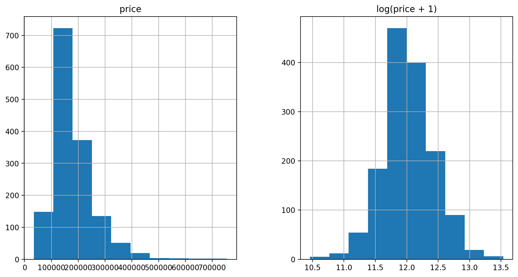
log transform the target:

train["SalePrice"] = np.log1p(train["SalePrice"])

log transform skewed numeric features:

numeric_feats = all_data.dtypes[all_data.dtypes != "object"].index

skewed_feats = train[numeric_feats].apply(lambda x: skew(x.dropna())) #compute skewness
skewed_feats = skewed_feats[skewed_feats > 0.75]
skewed_feats = skewed_feats.index

all_data[skewed_feats] = np.log1p(all_data[skewed_feats])

all_data = pd.get_dummies(all_data)

filling NA’s with the mean of the column:

all_data = all_data.fillna(all_data.mean())

Note that above I use all the data to compute the mean value that is then used for imputation. This is a flawed approach since it introduces some minor data leakage. However I decided to leave it here like this to showcase some common mistakes we all make :)

creating matrices for sklearn:

X_train = all_data[:train.shape[0]]
X_test = all_data[train.shape[0]:]
y = train.SalePrice

42.74.3. Models

Now we are going to use regularized linear regression models from the scikit learn module. I’m going to try both l_1(Lasso) and l_2(Ridge) regularization. I’ll also define a function that returns the cross-validation rmse error so we can evaluate our models and pick the best tuning par

from sklearn.linear_model import Ridge, RidgeCV, ElasticNet, LassoCV, LassoLarsCV
from sklearn.model_selection import cross_val_score

def rmse_cv(model):
    rmse= np.sqrt(-cross_val_score(model, X_train, y, scoring="neg_mean_squared_error", cv = 5))
    return(rmse)

model_ridge = Ridge()

The main tuning parameter for the Ridge model is alpha - a regularization parameter that measures how flexible our model is. The higher the regularization the less prone our model will be to overfit. However it will also lose flexibility and might not capture all of the signal in the data.

alphas = [0.05, 0.1, 0.3, 1, 3, 5, 10, 15, 30, 50, 75]
cv_ridge = [rmse_cv(Ridge(alpha = alpha)).mean() 
            for alpha in alphas]

cv_ridge = pd.Series(cv_ridge, index = alphas)
cv_ridge.plot(title = "Validation - Just Do It")
plt.xlabel("alpha")
plt.ylabel("rmse")

Text(0, 0.5, 'rmse')

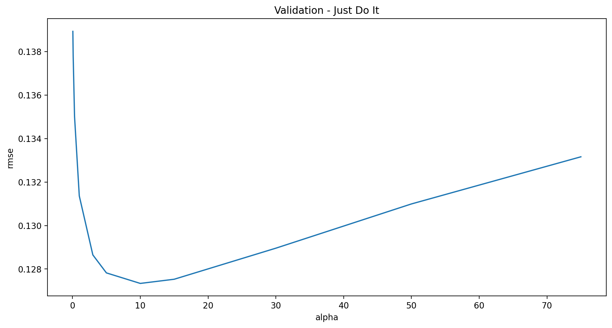
Note the U-ish shaped curve above. When alpha is too large the regularization is too strong and the model cannot capture all the complexities in the data. If however we let the model be too flexible (alpha small) the model begins to overfit. A value of alpha = 10 is about right based on the plot above.

cv_ridge.min()

0.12733734668670776

So for the Ridge regression we get a rmsle of about 0.127

Let’ try out the Lasso model. We will do a slightly different approach here and use the built in Lasso CV to figure out the best alpha for us. For some reason the alphas in Lasso CV are really the inverse or the alphas in Ridge.

model_lasso = LassoCV(alphas = [1, 0.1, 0.001, 0.0005]).fit(X_train, y)

rmse_cv(model_lasso).mean()

0.1225673588504812

Nice! The lasso performs even better so we’ll just use this one to predict on the test set. Another neat thing about the Lasso is that it does feature selection for you - setting coefficients of features it deems unimportant to zero. Let’s take a look at the coefficients:

coef = pd.Series(model_lasso.coef_, index = X_train.columns)

print("Lasso picked " + str(sum(coef != 0)) + " variables and eliminated the other " +  str(sum(coef == 0)) + " variables")

Lasso picked 110 variables and eliminated the other 178 variables

Good job Lasso. One thing to note here however is that the features selected are not necessarily the “correct” ones - especially since there are a lot of collinear features in this dataset. One idea to try here is run Lasso a few times on boostrapped samples and see how stable the feature selection is.

We can also take a look directly at what the most important coefficients are:

imp_coef = pd.concat([coef.sort_values().head(10),
                     coef.sort_values().tail(10)])

matplotlib.rcParams['figure.figsize'] = (8.0, 10.0)
imp_coef.plot(kind = "barh")
plt.title("Coefficients in the Lasso Model")

Text(0.5, 1.0, 'Coefficients in the Lasso Model')

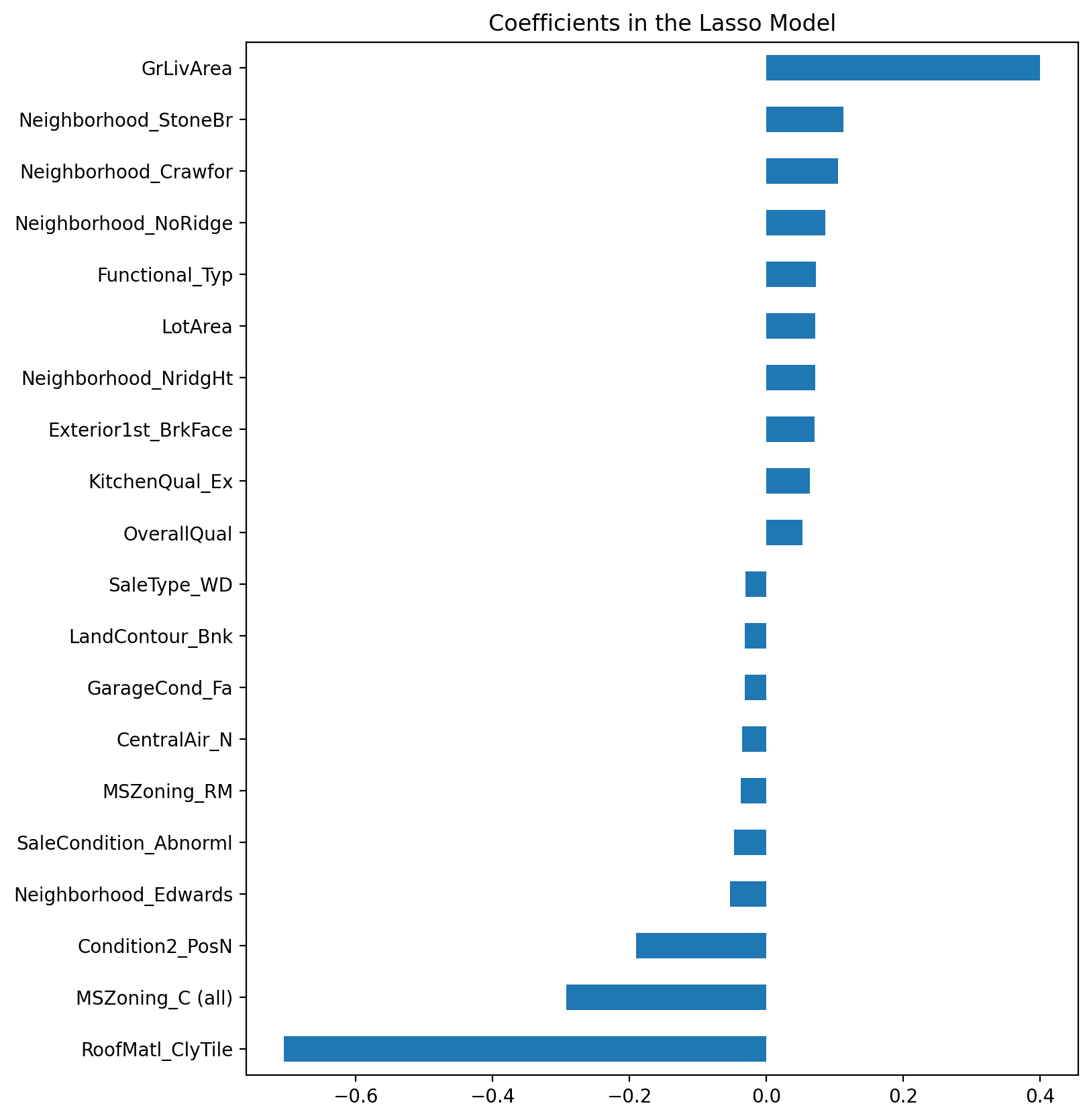
The most important positive feature is GrLivArea - the above ground area by area square feet. This definitely make sense. Then a few other location and quality features contributed positively. Some of the negative features make less sense and would be worth looking into more - it seems like they might come from unbalanced categorical variables.

Also note that unlike the feature importance you’d get from a random forest these are actual coefficients in your model - so you can say precisely why the predicted price is what it is. The only issue here is that we log_transformed both the target and the numeric features so the actual magnitudes are a bit hard to interpret and also the relationship is now multiplicative not additive.

let’s look at the residuals as well:

matplotlib.rcParams['figure.figsize'] = (6.0, 6.0)

preds = pd.DataFrame({"preds":model_lasso.predict(X_train), "true":y})
preds["residuals"] = preds["true"] - preds["preds"]
preds.plot(x = "preds", y = "residuals",kind = "scatter")

<Axes: xlabel='preds', ylabel='residuals'>

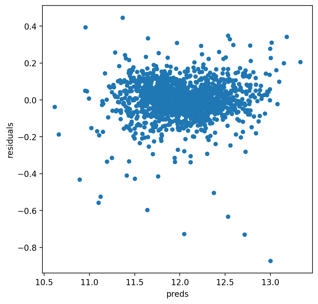
The residual plot looks pretty good.To wrap it up let’s predict on the test set and submit on the leaderboard:

42.74.4. Adding an xgboost model:

Let’s add an xgboost model to our linear model to see if we can improve our score:

import xgboost as xgb

dtrain = xgb.DMatrix(X_train, label = y)
dtest = xgb.DMatrix(X_test)

params = {"max_depth":2, "eta":0.1}
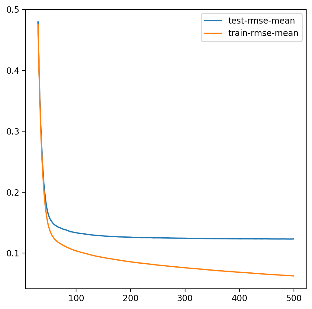
model = xgb.cv(params, dtrain,  num_boost_round=500, early_stopping_rounds=100)

model.loc[30:,["test-rmse-mean", "train-rmse-mean"]].plot()

<Axes: >

model_xgb = xgb.XGBRegressor(n_estimators=360, max_depth=2, learning_rate=0.1) #the params were tuned using xgb.cv
model_xgb.fit(X_train, y)

XGBRegressor(base_score=None, booster=None, callbacks=None,
             colsample_bylevel=None, colsample_bynode=None,
             colsample_bytree=None, early_stopping_rounds=None,
             enable_categorical=False, eval_metric=None, feature_types=None,
             gamma=None, gpu_id=None, grow_policy=None, importance_type=None,
             interaction_constraints=None, learning_rate=0.1, max_bin=None,
             max_cat_threshold=None, max_cat_to_onehot=None,
             max_delta_step=None, max_depth=2, max_leaves=None,
             min_child_weight=None, missing=nan, monotone_constraints=None,
             n_estimators=360, n_jobs=None, num_parallel_tree=None,
             predictor=None, random_state=None, ...)

In a Jupyter environment, please rerun this cell to show the HTML representation or trust the notebook.
On GitHub, the HTML representation is unable to render, please try loading this page with nbviewer.org.

xgb_preds = np.expm1(model_xgb.predict(X_test))
lasso_preds = np.expm1(model_lasso.predict(X_test))

predictions = pd.DataFrame({"xgb":xgb_preds, "lasso":lasso_preds})
predictions.plot(x = "xgb", y = "lasso", kind = "scatter")

<Axes: xlabel='xgb', ylabel='lasso'>

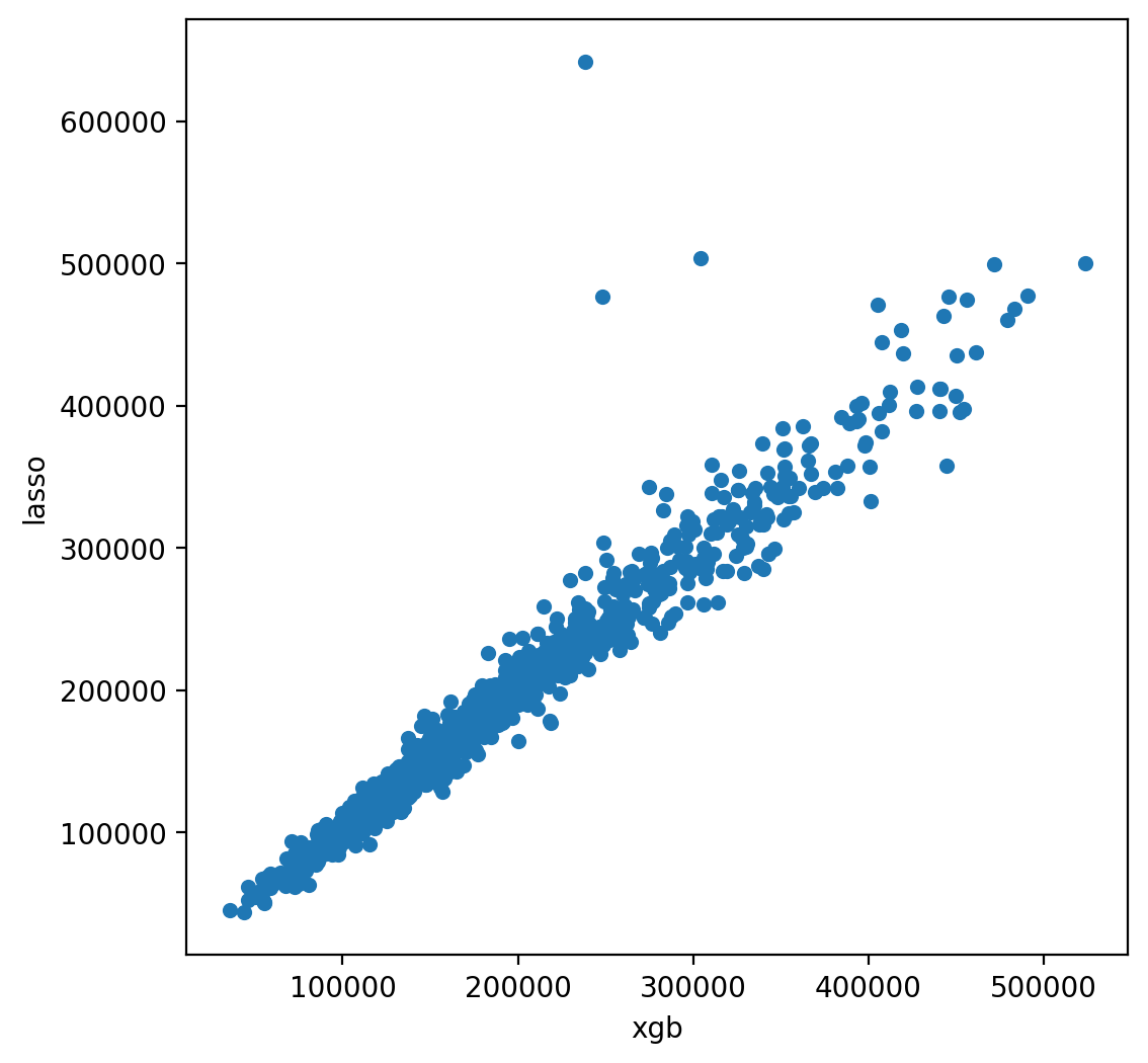
Many times it makes sense to take a weighted average of uncorrelated results - this usually imporoves the score although in this case it doesn’t help that much. Here we will just do a weighted average based on some randomly picked value. We could also do a CV grid search here as well.

preds = 0.7*lasso_preds + 0.3*xgb_preds

You can save it by following codes.

solution = pd.DataFrame({"id":test.Id, "SalePrice":preds})
solution.to_csv("ridge_sol.csv", index = False)

42.74.5. Acknowledgments

Thanks to Alexandru Papiu for creating the open-source project Regularized Linear Models. It inspires the majority of the content in this chapter.