# Install the necessary dependencies

import os
import sys
!{sys.executable} -m pip install --quiet seaborn pandas scikit-learn numpy matplotlib jupyterlab_myst ipython tensorflow tensorflow_addons

28. Image classification

28.1. What is image classification?

In this chapter we will introduce the image classification problem, which is the task of assigning an input image one label from a fixed set of categories. This is one of the core problems in Computer Vision that, despite its simplicity, has a large variety of practical applications.

from IPython.display import HTML
display(HTML("""
<p style="text-align: center;">
<iframe src="https://static-1300131294.cos.ap-shanghai.myqcloud.com/html/cls-demo/index.html" width="105%" height="700px;" style="border:none;"></iframe>
A demo of image classification. <a href="http://vision.stanford.edu/teaching/cs231n/">[source]</a>
</p>
"""))

A demo of image classification. [source]

Let me give you an example. In the image below an image classification model takes a single image and assigns probabilities to 4 labels, {cat, dog, hat, mug}. As shown in the image, keep in mind that to a computer an image is represented as one large 3-dimensional array of numbers. In this example, the cat image is 248 pixels wide, 400 pixels tall, and has three color channels Red,Green,Blue (or RGB for short). Therefore, the image consists of 248 x 400 x 3 numbers, or a total of 297,600 numbers. Each number is an integer that ranges from 0 (black) to 255 (white). Our task is to turn this quarter of a million numbers into a single label, such as “cat”.

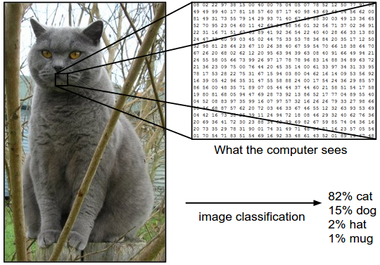
Fig. 28.1 Example of the image classification task

The task in image classification is to predict a single label (or a distribution over labels as shown here to indicate our confidence) for a given image. Images are 3-dimensional arrays of integers from 0 to 255, of size Width x Height x 3. The 3 represents the three color channels Red, Green, Blue.

28.2. Challenges

Since this task of recognizing a visual concept (e.g. cat) is relatively trivial for a human to perform, it is worth considering the challenges involved from the perspective of a Computer Vision algorithm. As we present (an inexhaustive) list of challenges below, keep in mind the raw representation of images as a 3-D array of brightness values:

• Viewpoint variation. A single instance of an object can be oriented in many ways with respect to the camera.

• Scale variation. Visual classes often exhibit variation in their size (size in the real world, not only in terms of their extent in the image).

• Deformation. Many objects of interest are not rigid bodies and can be deformed in extreme ways.

• Occlusion. The objects of interest can be occluded. Sometimes only a small portion of an object (as little as few pixels) could be visible.

• Illumination conditions. The effects of illumination are drastic on the pixel level.

• Background clutter. The objects of interest may blend into their environment, making them hard to identify.

• Intra-class variation. The classes of interest can often be relatively broad, such as chair. There are many different types of these objects, each with their own appearance.

A good image classification model must be invariant to the cross product of all these variations, while simultaneously retaining sensitivity to the inter-class variations.

28.3. Pipeline of image classification

We’ve seen that the task in image classification is to take an array of pixels that represents a single image and assign a label to it. Our complete pipeline can be formalized as follows:

• Input: Our input consists of a set of N images, each labeled with one of K different classes. We refer to this data as the training set,

• Learning: Our task is to use the training set to learn what every one of the classes looks like. We refer to this step as training a classifier, or learning a model,

• Evaluation: In the end, we evaluate the quality of the classifier by asking it to predict labels for a new set of images that it has never seen before. We will then compare the true labels of these images to the ones predicted by the classifier. Intuitively, we’re hoping that a lot of the predictions match up with the true answers (which we call the ground truth).

28.4. History & classic models

Since image classification is a classic task for computer vision, there are several models that are well-performed in the past. We can list them as follows: LeNet, AlexNet, VGGNet, GoogleNet, ResNet, DenseNet, SENet, MobileNet, ShuffleNet and ViT. In this part, we will introduce some of them.

28.4.1. VGGNet

The VGG (Visual Geometry Group) multilayer network model has 19 more layers than AlexNet, verifying that increasing the depth in the network structure can directly affect the model performance. The design idea of VGG is to increase the depth of the network and use a small size convolutional kernel instead. As shown in the figure below, three 3×3 convolutional kernels are used to replace the 7×7 convolutional kernels in AlexNet, and two 3×3 convolutional kernels are used to replace the 5×5 convolutional kernels, which can increase the depth of the network and improve the model effect while ensuring the same perceptual field. The number of model parameters and operations can be reduced by using smaller 3×3 Filters, and the image feature information can be better retained. The specific advantages of the improvement are summarized as follows.

• Using small 3×3 filters to replace large convolutional kernels.

• After replacing the convolution kernel, the convolution layers have the same perceptual field.

• Each layer is trained by ReLU activation function and batch gradient descent after convolution operation.

• It is verified that increasing the network depth can improve the model performance. Although, VGG has achieved good results in image classification and localization problems in 2014 due to its deeper network structure and low computational complexity, it uses 140 million parameters and is computationally intensive, which is its shortcoming.

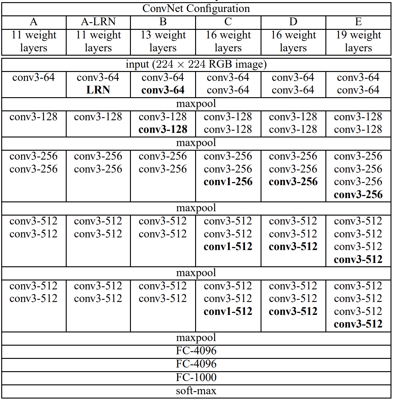
Fig. 28.2 Structure of VGGNet

28.4.1.1. Code

import numpy as np
import tensorflow as tf
import tensorflow_addons as tfa
import warnings

warnings.filterwarnings("ignore", category=DeprecationWarning)
AUTOTUNE = tf.data.experimental.AUTOTUNE

#This code defines a function `conv_bn` that returns a sequential model consisting of a zero-padding layer, 
# a convolution layer, and a batch normalization layer.

def conv_bn(out_channels, kernel_size, strides, padding, groups=1):
    return tf.keras.Sequential(
        [
            tf.keras.layers.ZeroPadding2D(padding=padding),
            tf.keras.layers.Conv2D(
                filters=out_channels,
                kernel_size=kernel_size,
                strides=strides,
                padding="valid",
                groups=groups,
                use_bias=False,
                name="conv",
            ),
            tf.keras.layers.BatchNormalization(name="bn"),
        ]
    )

This function is useful for constructing convolutional neural network architectures, as it provides a simple way to combine convolution and batch normalization layers.

• out_channels specifies the number of output channels for the convolution layer.

• kernel_size specifies the size of the convolution kernel.

• strides specifies the stride size for the convolution operation.

• padding specifies the padding size for the zero-padding layer.

• groups specifies the number of groups for the group convolution operation.

The function returns a sequential model that consists of three layers: a zero-padding layer, a convolution layer, and a batch normalization layer.

The convolution layer has out_channels filters, a kernel size of kernel_size, and a stride size of strides. The zero-padding layer has a padding size of padding. The batch normalization layer normalizes the activations of the convolution layer.

class RepVGGBlock(tf.keras.layers.Layer):
    def __init__(
        self,
        in_channels,
        out_channels,
        kernel_size,
        strides=1,
        padding=1,
        dilation=1,
        groups=1,
        deploy=False,
    ):
        super(RepVGGBlock, self).__init__()
        self.deploy = deploy
        self.groups = groups
        self.in_channels = in_channels

        assert kernel_size == 3
        assert padding == 1

        padding_11 = padding - kernel_size // 2

        self.nonlinearity = tf.keras.layers.ReLU()

        if deploy:
            self.rbr_reparam = tf.keras.Sequential(
                [
                    tf.keras.layers.ZeroPadding2D(padding=padding),
                    tf.keras.layers.Conv2D(
                        filters=out_channels,
                        kernel_size=kernel_size,
                        strides=strides,
                        padding="valid",
                        dilation_rate=dilation,
                        groups=groups,
                        use_bias=True,
                    ),
                ]
            )
        else:
            self.rbr_identity = (
                tf.keras.layers.BatchNormalization()
                if out_channels == in_channels and strides == 1
                else None
            )
            self.rbr_dense = conv_bn(
                out_channels=out_channels,
                kernel_size=kernel_size,
                strides=strides,
                padding=padding,
                groups=groups,
            )
            self.rbr_1x1 = conv_bn(
                out_channels=out_channels,
                kernel_size=1,
                strides=strides,
                padding=padding_11,
                groups=groups,
            )
            print("RepVGG Block, identity = ", self.rbr_identity)

    def call(self, inputs):
        if hasattr(self, "rbr_reparam"):
            return self.nonlinearity(self.rbr_reparam(inputs))

        if self.rbr_identity is None:
            id_out = 0
        else:
            id_out = self.rbr_identity(inputs)

        return self.nonlinearity(
            self.rbr_dense(inputs) + self.rbr_1x1(inputs) + id_out
        )

    # This func derives the equivalent kernel and bias in a DIFFERENTIABLE way.
    # You can get the equivalent kernel and bias at any time and do whatever you want,
    #     for example, apply some penalties or constraints during training, just like you do to the other models.
    # May be useful for quantization or pruning.
    def get_equivalent_kernel_bias(self):
        kernel3x3, bias3x3 = self._fuse_bn_tensor(self.rbr_dense)
        kernel1x1, bias1x1 = self._fuse_bn_tensor(self.rbr_1x1)
        kernelid, biasid = self._fuse_bn_tensor(self.rbr_identity)
        return (
            kernel3x3 + self._pad_1x1_to_3x3_tensor(kernel1x1) + kernelid,
            bias3x3 + bias1x1 + biasid,
        )

    def _pad_1x1_to_3x3_tensor(self, kernel1x1):
        if kernel1x1 is None:
            return 0
        else:
            return tf.pad(
                kernel1x1, tf.constant([[1, 1], [1, 1], [0, 0], [0, 0]])
            )

    def _fuse_bn_tensor(self, branch):
        if branch is None:
            return 0, 0
        if isinstance(branch, tf.keras.Sequential):
            kernel = branch.get_layer("conv").weights[0]
            running_mean = branch.get_layer("bn").moving_mean
            running_var = branch.get_layer("bn").moving_variance
            gamma = branch.get_layer("bn").gamma
            beta = branch.get_layer("bn").beta
            eps = branch.get_layer("bn").epsilon
        else:
            assert isinstance(branch, tf.keras.layers.BatchNormalization)
            if not hasattr(self, "id_tensor"):
                input_dim = self.in_channels // self.groups
                kernel_value = np.zeros(
                    (3, 3, input_dim, self.in_channels), dtype=np.float32
                )
                for i in range(self.in_channels):
                    kernel_value[1, 1, i % input_dim, i] = 1
                self.id_tensor = tf.convert_to_tensor(
                    kernel_value, dtype=np.float32
                )
            kernel = self.id_tensor
            running_mean = branch.moving_mean
            running_var = branch.moving_variance
            gamma = branch.gamma
            beta = branch.beta
            eps = branch.epsilon
        std = tf.sqrt(running_var + eps)
        t = gamma / std
        return kernel * t, beta - running_mean * gamma / std

    def repvgg_convert(self):
        kernel, bias = self.get_equivalent_kernel_bias()
        return kernel, bias

This code defines a RepVGGBlock layer in TensorFlow, which is a convolutional block used in the RepVGG model. The RepVGG model is a neural network architecture that achieves high accuracy while having a simple structure. The RepVGGBlock layer is designed to be more efficient and easier to train compared to other convolutional layers.

The RepVGGBlock layer has several parameters such as in_channels, out_channels, kernel_size, strides, padding, dilation, and groups. in_channels and out_channels determine the number of input and output channels, respectively.

• kernel_size specifies the size of the convolution kernel.

• strides determines the step size of the convolution operation.

• padding controls the amount of padding to be added to the input image.

• dilation specifies the dilation rate of the convolution operation.

• groups determines the number of groups to be used in the convolution operation.

The layer contains several convolutional operations, including a 3x3 convolution, a 1x1 convolution, and a residual identity. These convolutional operations are fused with batch normalization to improve training efficiency. The layer also includes a rectified linear unit (ReLU) activation function.

• The call() function of the RepVGGBlock layer applies the convolutional operations and the ReLU activation function to the input tensor.

• The get_equivalent_kernel_bias() function derives the equivalent kernel and bias of the layer in a differentiable way, which can be useful for applying penalties or constraints during training, such as in quantization or pruning.

• The repvgg_convert() function converts the RepVGGBlock layer to a standard convolutional layer by fusing batch normalization with convolutional operations.

class RepVGG(tf.keras.Model):
    def __init__(
        self,
        num_blocks,
        num_classes=1000,
        width_multiplier=None,
        override_groups_map=None,
        deploy=False,
    ):
        super(RepVGG, self).__init__()

        assert len(width_multiplier) == 4

        self.deploy = deploy
        self.override_groups_map = override_groups_map or dict()

        assert 0 not in self.override_groups_map

        self.in_planes = min(64, int(64 * width_multiplier[0]))

        self.stage0 = RepVGGBlock(
            in_channels=3,
            out_channels=self.in_planes,
            kernel_size=3,
            strides=2,
            padding=1,
            deploy=self.deploy,
        )
        self.cur_layer_idx = 1
        self.stage1 = self._make_stage(
            int(64 * width_multiplier[0]), num_blocks[0], stride=2
        )
        self.stage2 = self._make_stage(
            int(128 * width_multiplier[1]), num_blocks[1], stride=2
        )
        self.stage3 = self._make_stage(
            int(256 * width_multiplier[2]), num_blocks[2], stride=2
        )
        self.stage4 = self._make_stage(
            int(512 * width_multiplier[3]), num_blocks[3], stride=2
        )
        self.gap = tfa.layers.AdaptiveAveragePooling2D(output_size=1)
        self.linear = tf.keras.layers.Dense(num_classes)

    def _make_stage(self, planes, num_blocks, stride):
        strides = [stride] + [1] * (num_blocks - 1)
        blocks = []
        for stride in strides:
            cur_groups = self.override_groups_map.get(self.cur_layer_idx, 1)
            blocks.append(
                RepVGGBlock(
                    in_channels=self.in_planes,
                    out_channels=planes,
                    kernel_size=3,
                    strides=stride,
                    padding=1,
                    groups=cur_groups,
                    deploy=self.deploy,
                )
            )
            self.in_planes = planes
            self.cur_layer_idx += 1
        return tf.keras.Sequential(blocks)

    def call(self, x):
        out = self.stage0(x)
        out = self.stage1(out)
        out = self.stage2(out)
        out = self.stage3(out)
        out = self.stage4(out)
        out = self.gap(out)
        out = tf.keras.layers.Flatten()(out)
        out = self.linear(out)
        return out

This is a TensorFlow implementation of the RepVGG model, a type of convolutional neural network designed for efficient inference on mobile and embedded devices.

• The RepVGG model uses a series of RepVGG blocks to transform the input image into a feature representation that is then fed into a fully connected layer to make the final prediction.

• The RepVGG blocks are based on the VGG-style architecture, but instead of using traditional convolutional layers, they use a combination of 1x1 and 3x3 depthwise separable convolutions to reduce the number of parameters while maintaining performance.

• The width of the network can be adjusted by specifying a width multiplier for each stage of the network.

• The model also includes an adaptive average pooling layer to reduce the spatial dimensions of the feature map before the fully connected layer.

28.4.2. Resnet

ResNet (Residual Network) was proposed by Kaiming He and won the 2015 ILSVRC Grand Prix with an error rate of 3.57%. In the previous network, when the model is not deep enough, its network recognition is not strong, but when the network stack (Plain Network) is very deep, the network gradient disappearance and gradient dispersion are obvious, resulting in the model’s computational effectiveness but not up but down. Therefore, in view of the degradation problem of this deep network, ResNet is designed as an ultra-deep network without the gradient vanishing problem.ResNet has various types depending on the number of layers, from 18 to 1202 layers. As an example, Res Net50 consists of 49 convolutional layers and 1 fully connected layer, as shown in the figure below. This simple addition does not add additional parameters and computation to the network, but can greatly increase the training speed and improve the training effect, and this simple structure can well solve the degradation problem when the model deepens the number of layers. In this way, the network will always be in the optimal state and the performance of the network will not decrease with increasing depth.

The most important part of ResNet should be the residual block, and here is the structure.

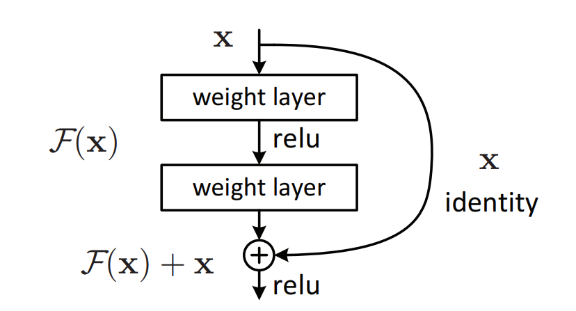
Fig. 28.3 Structure of residual block

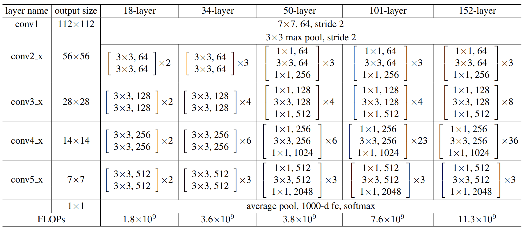
Fig. 28.4 Structure of residual network

28.4.2.1. Code

import tensorflow as tf

def conv_bn_relu(x, filters, kernel_size, strides=1):
    x = tf.layers.conv2d(x, filters, kernel_size, strides=strides, padding='same', use_bias=False)
    x = tf.layers.batch_normalization(x)
    x = tf.nn.relu(x)
    return x

def residual_block(x, filters, strides=1):
    shortcut = x
    x = conv_bn_relu(x, filters, kernel_size=3, strides=strides)
    x = conv_bn_relu(x, filters, kernel_size=3)
    x = x + shortcut
    return x

def resnet(input_shape, num_classes, num_filters=16, num_blocks=[3,3,3]):
    inputs = tf.placeholder(tf.float32, shape=[None, *input_shape])
    x = conv_bn_relu(inputs, num_filters, kernel_size=3)

    # Stacking residual blocks
    for i, num_blocks in enumerate(num_blocks):
        for j in range(num_blocks):
            strides = 1
            if j == 0 and i != 0:
                strides = 2
            x = residual_block(x, num_filters*(2**i), strides=strides)

    # Global average pooling and fully-connected layer for classification
    x = tf.reduce_mean(x, axis=[1,2])
    logits = tf.layers.dense(x, num_classes)

    return inputs, logits

This implementation uses the conv_bn_relu function to perform a convolution operation followed by batch normalization and ReLU activation.

• The residual_block function defines a residual block that consists of two convolutional layers with batch normalization and ReLU activation, followed by an addition of the input to the output of the second convolutional layer.

• The resnet function stacks multiple residual blocks and ends with a global average pooling layer and a fully-connected layer for classification.

28.4.3. DenseNet

DenseNet proposes a more radical dense connection mechanism than ResNet: i.e., connecting all layers to each other, specifically each layer accepts all the layers before it as its additional input. resNet short-circuits each layer with some previous layer (usually 2-3 layers), and the connection is made by element-level summation. In DenseNet, each layer is connected (concat) with all the preceding layers in the channel dimension and used as input to the next layer, which is a dense connection. Moreover, DenseNet is directly concat feature maps from different layers, which enables feature reuse and improves efficiency, and this feature is the most important difference between DenseNet and ResNet.

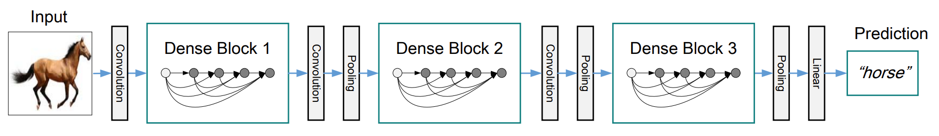
Fig. 28.5 Structure of dense block

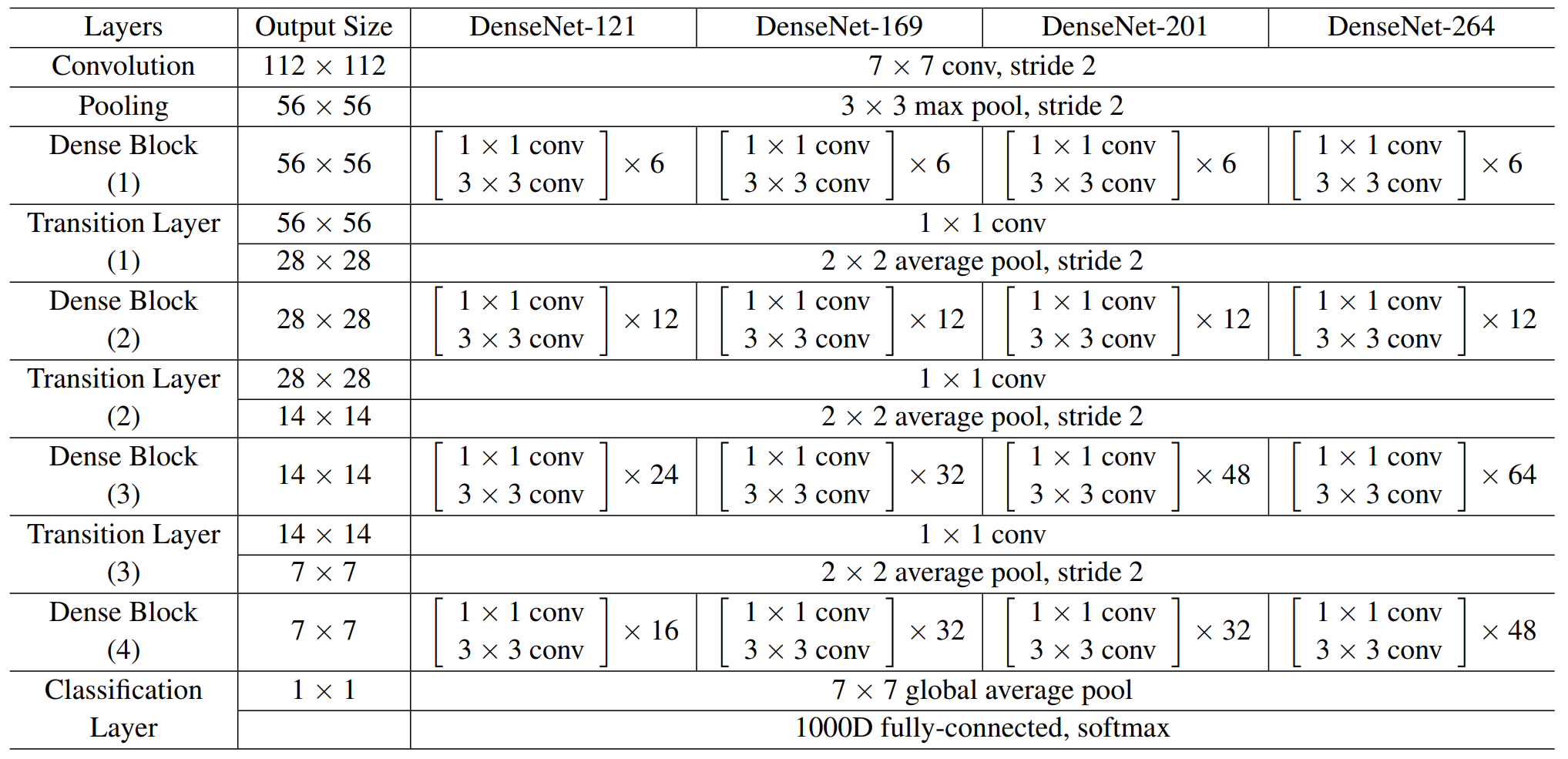
Fig. 28.6 Structure of dense network

28.4.3.1. Code

import tensorflow as tf

def conv_block(input, filters, dropout_rate):
    x = tf.layers.batch_normalization(input)
    x = tf.nn.relu(x)
    x = tf.layers.conv2d(x, filters, kernel_size=3, padding='same', activation=None)
    x = tf.layers.dropout(x, rate=dropout_rate)
    return x

def dense_block(input, n_layers, growth_rate, dropout_rate):
    for i in range(n_layers):
        conv = conv_block(input, growth_rate, dropout_rate)
        input = tf.concat([input, conv], axis=-1)
    return input

def transition_block(input, compression):
    n_filters = input.get_shape().as_list()[-1]
    n_filters = int(n_filters * compression)
    x = tf.layers.batch_normalization(input)
    x = tf.nn.relu(x)
    x = tf.layers.conv2d(x, n_filters, kernel_size=1, padding='same', activation=None)
    x = tf.layers.average_pooling2d(x, pool_size=2, strides=2, padding='valid')
    return x

def densenet(input, n_classes, n_dense_blocks=3, n_layers_per_block=4, growth_rate=12, compression=0.5, dropout_rate=0.2):
    # Initial convolution layer
    x = tf.layers.conv2d(input, filters=2*growth_rate, kernel_size=7, strides=2, padding='same', activation=None)
    x = tf.layers.batch_normalization(x)
    x = tf.nn.relu(x)
    x = tf.layers.max_pooling2d(x, pool_size=3, strides=2, padding='same')

    # Dense blocks
    for i in range(n_dense_blocks):
        x = dense_block(x, n_layers_per_block, growth_rate, dropout_rate)
        if i != n_dense_blocks-1:
            x = transition_block(x, compression)

    # Global average pooling and classification layer
    x = tf.layers.batch_normalization(x)
    x = tf.nn.relu(x)
    x = tf.layers.average_pooling2d(x, pool_size=x.get_shape().as_list()[1:3], strides=1)
    x = tf.layers.flatten(x)
    output = tf.layers.dense(x, units=n_classes, activation=None)
    
    return output

This implementation includes functions for building the building blocks of DenseNet: conv_block, dense_block, and transition_block. These building blocks are then used to construct the densenet function, which takes an input tensor and returns the output logits for a classification task.

The densenet function takes several hyperparameters as inputs, such as the number of dense blocks, the number of layers per block, the growth rate of each block, the compression factor for the transition blocks, and the dropout rate. These hyperparameters can be adjusted to optimize the performance of the model for a specific task.

28.4.4. MobileNet

MobileNets are based on a streamlined architecture that uses depth-wise separable convolutions to build light weight deep neural networks. We introduce two simple global hyper-parameters that efficiently trade off between latency and accuracy. These hyper-parameters allow the model builder to choose the right sized model for their application based on the constraints of the problem.

Besides, the standard convolutional filters for normal CNNs are replaced by two layers: depthwise convolution and pointwise convolution to build a depthwise separable filter.

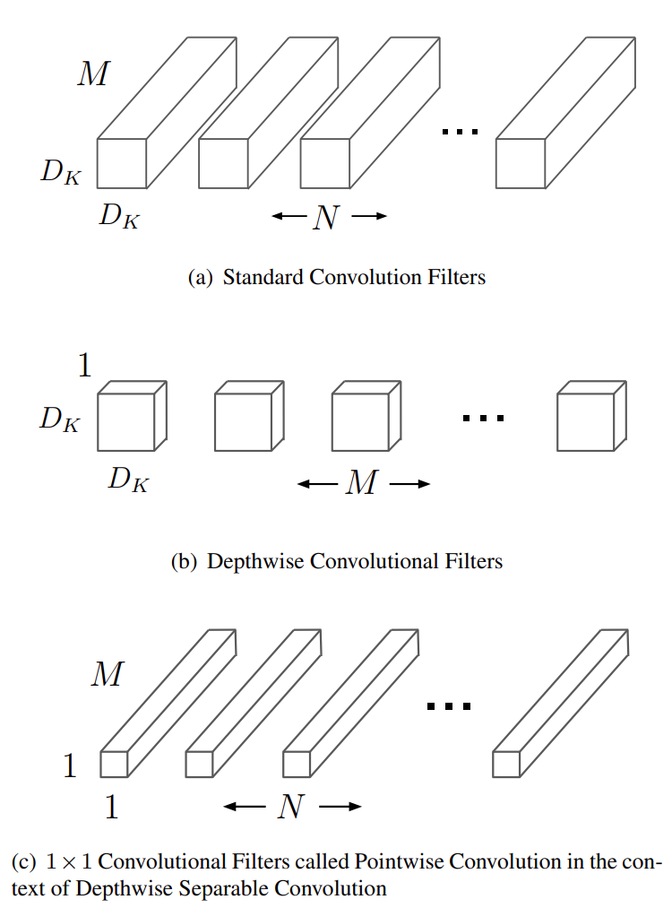
Fig. 28.7 Replacement of standard convolution filter

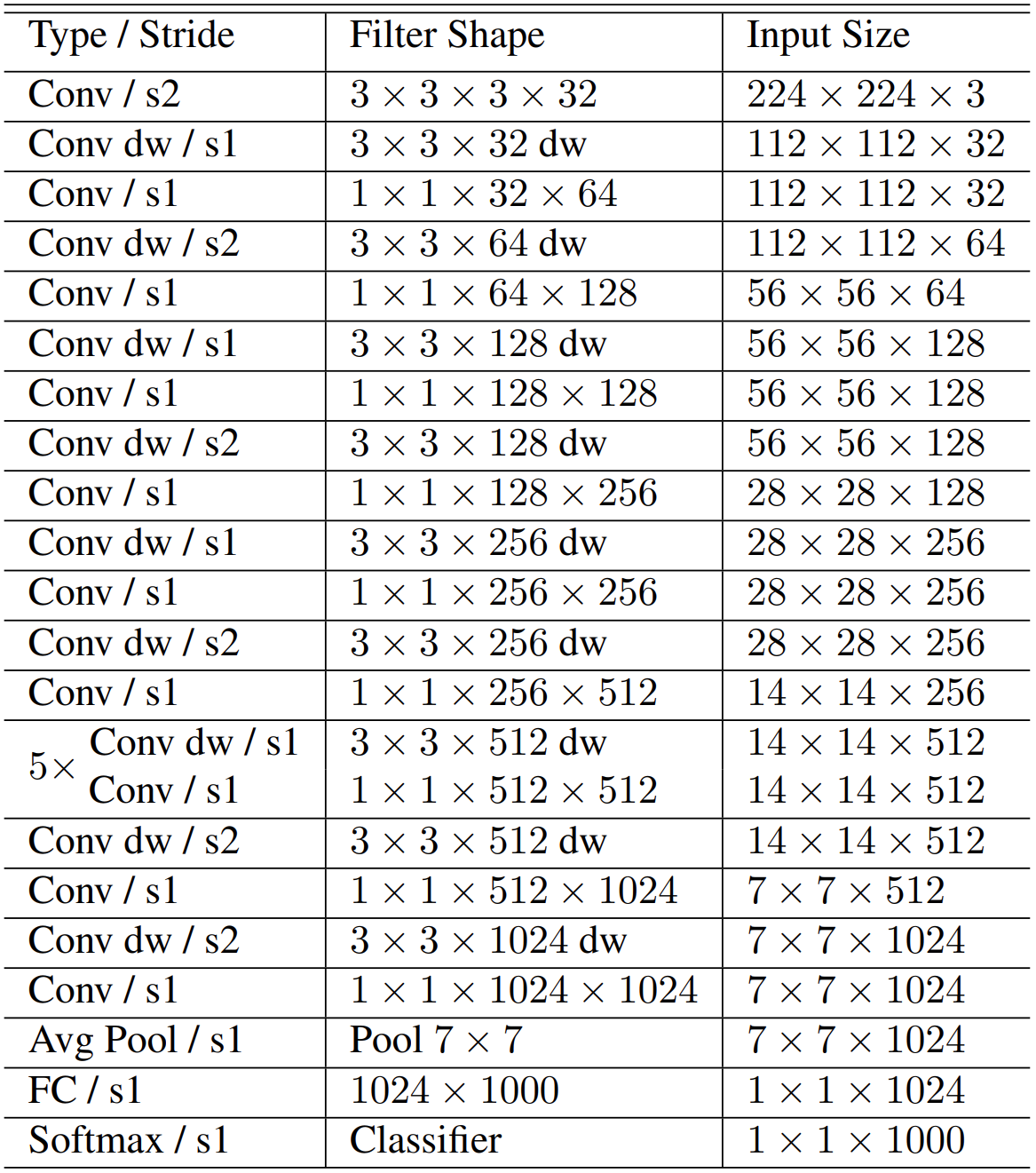
Fig. 28.8 Body structure of MobileNet

28.4.4.1. Code

import tensorflow as tf

def depthwise_separable_conv(inputs, num_filters, width_multiplier, downsample=False):
    """Depthwise Separable Convolution"""
    # Depthwise Convolution
    net = tf.keras.layers.DepthwiseConv2D(kernel_size=(3, 3), strides=(2 if downsample else 1, 2 if downsample else 1),
                                          depth_multiplier=width_multiplier, padding='same')(inputs)
    net = tf.keras.layers.BatchNormalization()(net)
    net = tf.keras.layers.ReLU()(net)

    # Pointwise Convolution
    net = tf.keras.layers.Conv2D(num_filters, kernel_size=(1, 1), strides=(1, 1), padding='same')(net)
    net = tf.keras.layers.BatchNormalization()(net)
    net = tf.keras.layers.ReLU()(net)

    return net

def mobilenet(input_shape, num_classes, width_multiplier=1):
    inputs = tf.keras.layers.Input(shape=input_shape)

    # Initial Convolution
    net = tf.keras.layers.Conv2D(int(32 * width_multiplier), kernel_size=(3, 3), strides=(2, 2), padding='same')(inputs)
    net = tf.keras.layers.BatchNormalization()(net)
    net = tf.keras.layers.ReLU()(net)

    # Depthwise Separable Convolution x 13
    net = depthwise_separable_conv(net, int(64 * width_multiplier), width_multiplier)
    net = depthwise_separable_conv(net, int(128 * width_multiplier), width_multiplier, downsample=True)
    net = depthwise_separable_conv(net, int(128 * width_multiplier), width_multiplier)
    net = depthwise_separable_conv(net, int(256 * width_multiplier), width_multiplier, downsample=True)
    net = depthwise_separable_conv(net, int(256 * width_multiplier), width_multiplier)
    net = depthwise_separable_conv(net, int(512 * width_multiplier), width_multiplier, downsample=True)
    for i in range(5):
        net = depthwise_separable_conv(net, int(512 * width_multiplier), width_multiplier)
    net = depthwise_separable_conv(net, int(1024 * width_multiplier), width_multiplier, downsample=True)
    net = depthwise_separable_conv(net, int(1024 * width_multiplier), width_multiplier)
    net = tf.keras.layers.GlobalAveragePooling2D()(net)

    # Output
    outputs = tf.keras.layers.Dense(num_classes, activation='softmax')(net)

    return tf.keras.models.Model(inputs=inputs, outputs=outputs)

This implementation defines two functions: depthwise_separable_conv and mobilenet. The former implements the depthwise separable convolution operation used by the MobileNet architecture, while the latter constructs the entire MobileNet model.

The mobilenet function takes three arguments: input_shape (a tuple specifying the input shape of the model), num_classes (the number of output classes), and width_multiplier (a scaling factor for the number of filters in each layer of the model, defaulting to 1).

28.4.5. ViT

Different from the previous models, ViT (Vision Transformer) uses the concept of Transformer. Inspired by the Transformer scaling successes in NLP, they experiment with applying a standard Transformer directly to images, with the fewest possible modifications. To do so, they split an image into patches and provide the sequence of linear embeddings of these patches as an input to a Transformer. Image patches are treated the same way as tokens (words) in an NLP application. They train the model on image classification in supervised fashion.

28.4.5.1. Code

import tensorflow as tf
from tensorflow.keras.layers import LayerNormalization, MultiHeadAttention, Dense, Dropout, Input
from tensorflow.keras.layers.experimental.preprocessing import Resizing
from tensorflow.keras.models import Model


class TransformerBlock(tf.keras.layers.Layer):
    def __init__(self, embed_dim, num_heads, ff_dim, rate=0.1):
        super(TransformerBlock, self).__init__()
        self.att = MultiHeadAttention(num_heads=num_heads, key_dim=embed_dim)
        self.ffn = tf.keras.Sequential([
            Dense(ff_dim, activation='relu'),
            Dense(embed_dim),
        ])
        self.layernorm1 = LayerNormalization(epsilon=1e-6)
        self.layernorm2 = LayerNormalization(epsilon=1e-6)
        self.dropout1 = Dropout(rate)
        self.dropout2 = Dropout(rate)

    def call(self, inputs, training):
        attn_output = self.att(inputs, inputs)
        attn_output = self.dropout1(attn_output, training=training)
        out1 = self.layernorm1(inputs + attn_output)
        ffn_output = self.ffn(out1)
        ffn_output = self.dropout2(ffn_output, training=training)
        return self.layernorm2(out1 + ffn_output)


class VisionTransformer(tf.keras.Model):
    def __init__(self, image_size, patch_size, num_layers, num_heads, ff_dim, num_classes, rate=0.1):
        super(VisionTransformer, self).__init__()
        num_patches = (image_size // patch_size) ** 2
        self.patch_dim = 3 * patch_size ** 2
        self.reshape = Resizing(image_size, interpolation='bilinear')
        self.patchify = tf.keras.layers.experimental.preprocessing.Patching(num_patches)
        self.patch_projection = Dense(units=self.patch_dim, activation='linear')
        self.position_embedding = self.add_weight('position_embedding', shape=(1, num_patches + 1, self.patch_dim),
                                                   initializer=tf.keras.initializers.RandomNormal(),
                                                   trainable=True)
        self.dropout = Dropout(rate)
        self.transformer_blocks = [TransformerBlock(embed_dim=self.patch_dim, num_heads=num_heads, ff_dim=ff_dim, rate=rate)
                                   for _ in range(num_layers)]
        self.layernorm = LayerNormalization(epsilon=1e-6)
        self.classifier = Dense(units=num_classes, activation='softmax')

    def call(self, inputs, training):
        x = self.reshape(inputs)
        x = self.patchify(x)
        x = self.patch_projection(x)
        x = tf.concat([tf.zeros((tf.shape(x)[0], 1, self.patch_dim)), x], axis=1)
        x += self.position_embedding
        x = self.dropout(x, training=training)
        for transformer_block in self.transformer_blocks:
            x = transformer_block(x, training)
        x = self.layernorm(x)
        x = x[:, 0]
        return self.classifier(x)

The above code defines a Vision Transformer (ViT) model in TensorFlow, which is a state-of-the-art architecture for image classification tasks that combines the transformer architecture with a patch-based approach for image processing.

The TransformerBlock class defines a single transformer block with multi-head attention and a feedforward neural network. The constructor takes in the following arguments:

• embed_dim: the dimensionality of the embedding layer

• num_heads: the number of attention heads

• ff_dim: the dimensionality of the feedforward layer

• rate: the dropout rate

The call method of the TransformerBlock class takes in the input tensor and a boolean flag training indicating whether the layer should behave in training or inference mode. The input tensor is passed through the multi-head attention layer, followed by a dropout layer, and then added to the input tensor using residual connections. The resulting tensor is passed through a feedforward neural network, followed by another dropout layer, and then added to the residual tensor using another residual connection.

The VisionTransformer class defines the ViT model, which consists of multiple transformer blocks and a final dense layer for classification. The constructor takes in the following arguments:

• image_size: the size of the input image

• patch_size: the size of the patches to be extracted from the image

• num_layers: the number of transformer blocks in the model

• num_heads: the number of attention heads in each transformer block

• ff_dim: the dimensionality of the feedforward layer in each transformer block

• num_classes: the number of output classes

• rate: the dropout rate

The call method of the VisionTransformer class takes in the input tensor and a boolean flag training indicating whether the layer should behave in training or inference mode. The input tensor is first resized to the specified image_size and then passed through a patch extraction layer that divides the image into patches of size patch_size. Each patch is projected to a patch_dim-dimensional embedding space using a dense layer. A learnable position embedding is added to the patches and the resulting tensor is passed through a dropout layer. The resulting tensor is then passed through a stack of num_layers transformer blocks, each followed by a dropout layer. The output of the final transformer block is passed through a layer normalization layer and the first element of the resulting tensor is passed through a dense layer with num_classes output units and a softmax activation function.

28.5. Classic datasets

As we said before, image classification task is mainly trained by datasets, so the importance of dataset is obvious. Here, we will introduce some widely-used datasets.

28.5.1. CIFAR-10/100

The CIFAR-10 dataset consists of 60000 32x32 colour images in 10 classes, with 6000 images per class. There are 50000 training images and 10000 test images. The dataset is divided into five training batches and one test batch, each with 10000 images. The test batch contains exactly 1000 randomly-selected images from each class. The training batches contain the remaining images in random order, but some training batches may contain more images from one class than another. Between them, the training batches contain exactly 5000 images from each class.

The CIFAR-100 dataset is just like the CIFAR-10, except it has 100 classes containing 600 images each. There are 500 training images and 100 testing images per class. The 100 classes in the CIFAR-100 are grouped into 20 superclasses. Each image comes with a “fine” label (the class to which it belongs) and a “coarse” label (the superclass to which it belongs).

Note

Download for Linux wget http://www.cs.toronto.edu/~kriz/cifar-10-python.tar.gz wget http://www.cs.toronto.edu/~kriz/cifar-100-python.tar.gz

Download for Win/Mac Download from the offical website

28.5.2. ImageNet-1000

ImageNet is an image dataset organized according to the WordNet hierarchy. Each meaningful concept in WordNet, possibly described by multiple words or word phrases, is called a “synonym set” or “synset”. There are more than 100,000 synsets in WordNet; the majority of them are nouns (80,000+). In ImageNet, we aim to provide on average 1000 images to illustrate each synset. Images of each concept are quality-controlled and human-annotated. In its completion, we hope ImageNet will offer tens of millions of cleanly labeled and sorted images for most of the concepts in the WordNet hierarchy.

Note

If you want to download this dataset, please visit kaggle for more information.

28.6. Standards

28.6.1. Top-1 accuracy

If your predicted label takes the largest one inside the final probability vector as the prediction result, and if the one with the highest probability in your prediction result is correctly classified, then the prediction is correct. Otherwise, the prediction is wrong.

28.6.2. Top-5 accuracy

Among the 50 classification probabilities of the test image, take the first 5 maximum classification probabilities, whether the correct label (classification) is in it or not, that is, whether it is one of these first 5, if it is, it is a successful classification.

28.7. Your turn! 🚀

Assignment - Image classification

28.8. Acknowledgments

Thanks to Stanford for creating the open-source course CS231n: Deep Learning for Computer Vision, Duc Thang HOANG for creating the open-source project RepVGG-Tensorflow-2, Junho Kim for creating the open-source project ResNet-Tensorflow, Densenet-Tensorflow and vit-tensorflow and ohadlights for creating the open-source project mobilenetv2. They inspire the majority of the content in this chapter.