42.80. Hyperparameter tuning gradient boosting#

42.80.1. Context:#

A company which is active in Big Data and Data Science wants to hire data scientists among people who successfully pass some courses which are conducted by the company. Many people sign up for their training. Company wants to know which of these candidates really want to work for the company after training, because it helps reducing the cost and time as well as increasing the quality of training and the planning of the courses. Information related to demographics, education, experience are in hands from candidates signup and enrollment.

42.80.2. Features#

enrollee_id : Unique ID for candidate
city: City code
city_ development _index : Developement index of the city (scaled)
gender: Gender of candidate
relevent_experience: Relevant experience of candidate
enrolled_university: Type of University course enrolled if any
education_level: Education level of candidate
major_discipline :Education major discipline of candidate
experience: Candidate total experience in years
company_size: No of employees in current employer’s company
company_type : Type of current employer
lastnewjob: Difference in years between previous job and current job
training_hours: training hours completed
target: 0 – Not looking for job change, 1 – Looking for a job change

42.80.3. Plan:#

We will treat each column in two phases:

42.80.3.1. Data preprocessing:#

Imputing missing values.
Handling categorical data.

42.80.3.2. Data Visualization#

42.80.3.3. Model Creation:#

Then we will test several model and choose the one with the best performance:

Models: Logistic Regression-SVM-Gradient Boosting-KNN-RandomForest-XGBoost classifier.
Hyperparameter tuning.
Use the model to predict target column in Test set.

42.80.4. Imports¶#

Lets get started, first lets import our typical libraries:

import numpy as np
import pandas as pd 
import seaborn as sns
import matplotlib.pyplot as plt
import warnings

warnings.filterwarnings("ignore")

import os
for dirname, _, filenames in os.walk('/kaggle/input'):
    for filename in filenames:
        print(os.path.join(dirname, filename))
print("Setup complete")

42.80.5. Loading the data#

Let’s import our train and test data.

#Data
train = pd.read_csv("../../../assets/data/aug_train.csv")

#testing data
#test = pd.read_csv('../input/hr-analytics-job-change-of-data-scientists/aug_test.csv')

Let’s take a closer look to our data.

train.head()

From the first glence we can see that most of the data is categorical, and we have several missing values in different columns. Let’s take a look at the number of missing values in each column:

print("Train data missing values: \n",train.isna().sum())

train.count()

42.80.6. Exploratory data analysis#

42.80.6.1. Task 1: City#

train["city"].unique()

We can see that every city has a specific number, with a prefix “city_”, so first we have to delete the prefix then transform the data from object type to integer.

train['city'] = train['city'].map(lambda row: row.replace('city_',''))

train['city'] = train['city'].astype(int)

The result of cities

print(train["city"].unique())
print("We have {} unique variables:".format(len(train["city"].unique())))

plt.figure(figsize=(16,8))
g = sns.distplot(train.city,kde=False, color="red")
g = (g.set(xlim=(0,185),xticks=range(0,190,10)))
plt.xlabel("City Number")
plt.ylabel("Distribution")
plt.show()

print("Most common cities are:\n",train['city'].value_counts())

We can see that candidates from the city number 103 are the majority.

train.sort_values(by='city')

And here we can see that each city has specific city_development_index, so deleting this column won’t make any difference to the model, however we can visualize what is the development index for the cities with the majority of candidates:

train.loc[train.city == 103,'city_development_index']

So the city with the majority of candidates is a well developped city, but do we have a relationship between the city development index and the chance of the candidate looking for another job?

train['city'] = train['city'].astype(np.int8)

sns.lineplot(x='target', y='city_development_index',data=train)
plt.show()

The candidates from cities with low development index tend to look for a job change and vice versa. Now let’s just drop this column.

train = train.drop(labels='city_development_index', axis=1)

42.80.6.2. Task2: Gender#

It is obvious we have to encode the caregorical data and take care of missing data, there are a lot of ways to handle gender missing values such as replacing them with most common gender in the dataset, deleting those rows…etc. But I prefer to fill the gender missing values with “Other” since we may have candidates identify as non-binary. First lets take a look at our gender column:

plt.figure(figsize=(12,6))
sns.violinplot(x='gender', y='target', palette='Set2', data=train)
plt.show()

It looks like more men don’t look for a job change but actually we can’t conclude that from this violinplot since most of the candidates are men.

train['gender'].hist()
plt.show()

Now let’s fill the missing values with ‘Other’:

train['gender'] = train['gender'].fillna('Other')

Since we don’t have any missing values left in the gender column, let’s encode the column, I will use for this one LabelEncoder of sklearn:

from sklearn.preprocessing import LabelEncoder

label_encoder = LabelEncoder()
train["gender"] = label_encoder.fit_transform(train["gender"])

Female : 0
Male : 1
Other : 2

Lets have a look at what we have achieved so far:

train.isna().sum()

train.head()

42.80.6.3. Task 3：Relevant experience#

Before making any decision we have to look at the values of this column:

train['relevent_experience'].unique()

So it only has two values, and no missing data.

Encoding:

train["relevent_experience"] = train["relevent_experience"].map({"Has relevent experience":1, "No relevent experience":0})

42.80.6.4. Encoding:#

train["relevent_experience"] = train["relevent_experience"].map({"Has relevent experience":1, "No relevent experience":0})

42.80.6.5. Task 4: Enrolled university#

train['enrolled_university'].unique()

This column has missing values, lets take care of them before encoding.

sns.countplot(x='enrolled_university', data=train)
plt.show()

Most of the candidates had no university enrollment

sns.lineplot(x='enrolled_university', y='target', palette='Set2', data=train)
plt.show()

We can see that most of candidates had no enrollment more likely aren’t looking for a job change.

We can’t tell if the missing data is left out or the candidates had no enrollment, but also we don’t want to create a new value (like ‘OTHER’) because it can create a pattern that doesn’t exist. I will fill the missing values with the no_enrollment value.

train["enrolled_university"]=train["enrolled_university"].fillna('no_enrollment')

Encode:

train["enrolled_university"] = label_encoder.fit_transform(train["enrolled_university"])

42.80.6.6. Task 5: Education level#

train['education_level'].unique()

train['education_level'].hist()
plt.show()

Most candidates are graduates.

sns.lineplot(x='education_level', y='target', palette='Set2', data=train)
plt.show()

Graduates and Masters are most likely to look for a job change, but people with Phd or primary school aren’t.

train["education_level"]=train["education_level"].fillna('Other')

train["education_level"] = label_encoder.fit_transform(train["education_level"])

42.80.6.7. Task 6: Major discipline#

train['major_discipline'].unique()

STEM: Science, technology, engineering, and mathematics

train['major_discipline'].hist()

Most of our candidates are STEM majors.

train['major_discipline'] = train['major_discipline'].fillna('Other')

train["major_discipline"] = label_encoder.fit_transform(train["major_discipline"])

train.head()

42.80.6.8. Task 7: Experience#

The experience variable is an object indicating the minimum or maximum years of experience a candidate had, so deleting the operators won’t make a big difference.

First we have to convert the column to string.

train['experience'] = train['experience'].astype(str)

train['experience'] = train['experience'].apply(lambda col: col.replace('>',''))
train['experience'] = train['experience'].apply(lambda col: col.replace('<',''))

Delete the symbols.

train.head()

Lets fill the missing values with 0.

train['experience'] = train['experience'].apply(lambda col: col.replace('nan','0'))

Convert the values to Integer.

train['experience'] = pd.to_numeric(train['experience'])

42.80.6.9. Task 8:Company size#

train['company_size'].unique()

We have 5938 missing values in the company_size column, before encoding categorical data we have to handle the missing values.

sns.countplot(y='company_size', data=train)
plt.show()

42.80.6.9.1. We can see that most candidates work in small companies (between 50-500)#

Identify each interval with a number:

train['company_size'] = train['company_size'].map({"50-99":0, "<10":1, "10000+":2, "5000-9999":3, "1000-4999":4, "10/49":5, "100-500":6, "500-999":7})

train.shape

30% of candidates didn’t mention if they had experience or not, so we will assume that these candidates have no experience.

train['company_size'] = train['company_size'].fillna(8)

42.80.6.10. Task 9:Company type#

sns.countplot(y='company_type', data=train)
plt.show()

Most of candidates work in Private limited company type (pvt ltd)

train['company_type'] = train['company_type'].map({"Pvt Ltd":0, "Funded Startup":1, "Early Stage Startup":2, "Public Sector":3, "NGO":4, "Other":5})

plt.figure(figsize=(12,6))
sns.violinplot(x='company_size', y='company_type',data=train)
plt.show()

Private limited companies are of different sizes, from less than ten people to +10 000! So we can’t really find a relation between company size and type. We will fill missing values in company_type with 0(private limited comapany).

train['company_type'] = train['company_type'].fillna(0)

42.80.6.11. Task 10: Last new job#

train['last_new_job'].unique()

We assume that missing values are from candidates that had no job.

train['last_new_job'] = train['last_new_job'].fillna('never')

train['last_new_job'] = train['last_new_job'].map({"1":1, ">4": 5, "never":0, "4":4, "3":3, "2":2})

g = sns.catplot(y="target",x="last_new_job",data=train, kind="bar")

So we have taken care of all categorical data and missing values, lets take a look at what we have done so far:

train.head()

train.dtypes

42.80.6.12. Task 11: Pre modeling steps#

pred = train['target']

train = train.drop(labels='target', axis=1)

train = train.astype(np.int8)

42.80.7. Models testing#

from sklearn.pipeline import Pipeline
from sklearn import svm
from sklearn.linear_model import LogisticRegression
from sklearn.ensemble import RandomForestClassifier, AdaBoostClassifier
import xgboost as xgb
from sklearn.neighbors import KNeighborsClassifier
from sklearn.ensemble import GradientBoostingClassifier
from sklearn import metrics
from sklearn.model_selection import KFold, cross_val_score, train_test_split

Lets try different models and see what works best:

KFold_Score = pd.DataFrame()
classifiers = ['Linear SVM', 'LogisticRegression', 'RandomForestClassifier', 'XGBoostClassifier','GradientBoostingClassifier']
models = [svm.SVC(kernel='linear'),
          LogisticRegression(max_iter = 1000),
          RandomForestClassifier(n_estimators=200, random_state=0),
          xgb.XGBClassifier(n_estimators=100),
          GradientBoostingClassifier(random_state=0)
         ]

j = 0
for i in models:
    model = i
    cv = KFold(n_splits=5, random_state=0, shuffle=True)
    KFold_Score[classifiers[j]] = (cross_val_score(model, train, np.ravel(pred), scoring = 'accuracy', cv=cv))
    j = j+1

mean = pd.DataFrame(KFold_Score.mean(), index= classifiers)
KFold_Score = pd.concat([KFold_Score,mean.T])
KFold_Score.index=['Fold 1','Fold 2','Fold 3','Fold 4','Fold 5','Mean']
KFold_Score.T.sort_values(by=['Mean'], ascending = False)

Obviously,Gradient Boosting gives the best result.

42.80.8. Boosting:#

Ensemble learning techniques: They combine the predictions of multiple machine learning models.

Boosting: Boosting algorithms play a crucial role in dealing with bias variance trade-off. Unlike bagging algorithms, which only controls for high variance in a model, boosting controls both the aspects (bias & variance), and is considered to be more effective. Boosting is an ensemble learning technique.

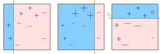
Boosting is a sequential technique which works on the principle of ensemble. It combines a set of weak learners and delivers improved prediction accuracy. At any instant t, the model outcomes are weighed based on the outcomes of previous instant t-1. The outcomes predicted correctly are given a lower weight and the ones miss-classified are weighted higher.

Visually:

42.80.9. Gradient Boosting:#

The overall parameters of gradient boosting can be devided into three categories:

Tree-Specific Parameters: These affect each individual tree in the model.
Boosting Parameters: These affect the boosting operation in the model.
Miscellaneous Parameters: Other parameters for overall functioning.

42.80.9.1. Tree-specific parameters#

42.80.9.2. Boosting parameters:#

learning_rate
n_estimators
subsample

42.80.9.3. Miscellaneous parameters#

loss
init
random_state
verbose

Boosting reference: https://www.analyticsvidhya.com/blog/2016/02/complete-guide-parameter-tuning-gradient-boosting-gbm-python/

Patrick Winston, MIT: https://www.youtube.com/watch?v=UHBmv7qCey4

42.80.10. Hyperparameter Tuning using GridSearchCV#

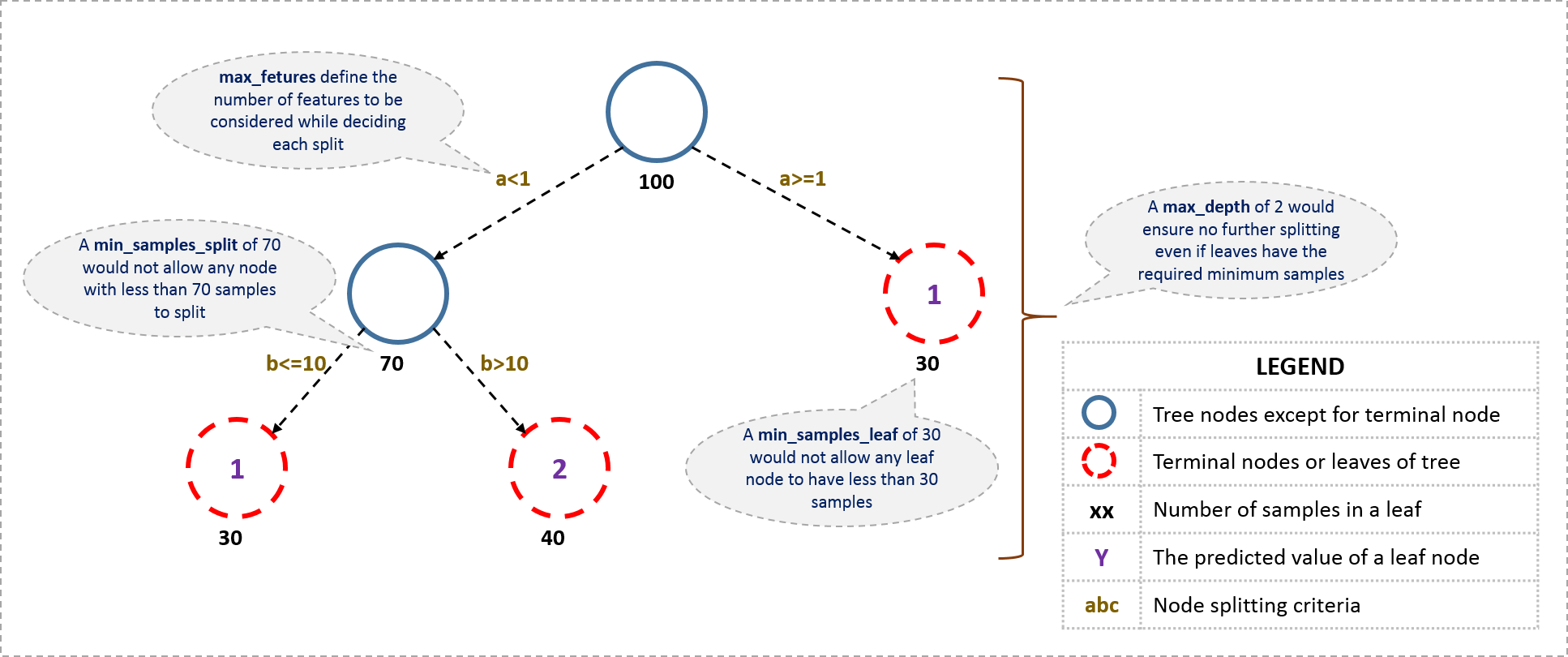
GradientBoostingClassifier(*, loss=‘deviance’, learning_rate=0.1, n_estimators=100, subsample=1.0, criterion=‘friedman_mse’, min_samples_split=2, min_samples_leaf=1, min_weight_fraction_leaf=0.0, max_depth=3, min_impurity_decrease=0.0, min_impurity_split=None, init=None, random_state=None, max_features=None, verbose=0, max_leaf_nodes=None, warm_start=False, validation_fraction=0.1, n_iter_no_change=None, tol=0.0001, ccp_alpha=0.0)

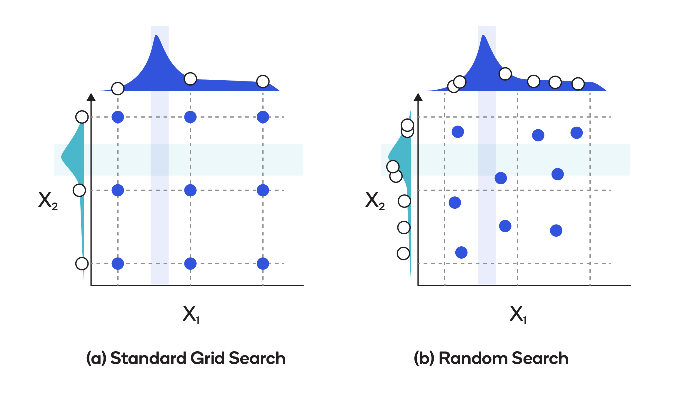
Grid search is best described as exhuastive guess and check. We have a problem: find the hyperparameters that result in the best cross validation score, and a set of values to try in the hyperparameter grid - the domain. The grid search method for finding the answer is to try all combinations of values in the domain and hope that the best combination is in the grid (in reality, we will never know if we found the best settings unless we have an infinite hyperparameter grid which would then require an infinite amount of time to run).

Grid search suffers from one limiting problem: it is extremely computationally expensive because we have to perform cross validation with every single combination of hyperparameters in the grid!

Pros:

We don’t have to write a long (nested for loops) code.
Finds the best model within the grid.

Cons:

Computationally expensive.
It is ‘uninformed’. Results of one model don’t help creating the next model.

42.80.10.1. Task 1: Initialize model#

X_train, X_test, y_train, y_test = train_test_split(train, pred, test_size=0.3, random_state=42)

Lets initialize our model with these parameters:

y_train.head()

mymodel = GradientBoostingClassifier(learning_rate=0.1, min_samples_split=500,min_samples_leaf=50,max_depth=8,max_features='sqrt',subsample=0.8,random_state=10)

42.80.10.2. Task 2: Remove enrollee_id#

We shouldn’t use the enrollee_id since it is unique for each candidate.

predictors = [x for x in X_train.columns if x not in ["enrollee_id"]]

predictors

42.80.10.3. Task 3: Look for optimal number#

First we have to look for an optimal number of estimators:

param_test1 = {'n_estimators':range(10,100,10)}

Grid search:

from sklearn.model_selection import GridSearchCV
CV_gbc = GridSearchCV(estimator=mymodel, param_grid=param_test1, scoring='roc_auc',n_jobs=4, cv= 5)
CV_gbc.fit(X_train[predictors],y_train)
CV_gbc.best_params_, CV_gbc.best_score_

CV_gbc.cv_results_

dir(CV_gbc)

42.80.10.4. Task 4: Find learning rate#

As you can see that here we got 90 as the optimal estimators for 0.1 learning rate, it is close to 100 so we will increase the learning rate to 0.2. (I tried working with number of estimators as 90 but when I increased the learning rate I got slightly better results, I won’t include the whole process because it will take a lot of time to run)

mymodel0 = GradientBoostingClassifier(learning_rate=0.2, min_samples_split=500,min_samples_leaf=50,max_depth=8,max_features='sqrt',subsample=0.8,random_state=10)

from sklearn.model_selection import GridSearchCV
CV_gbc0 = GridSearchCV(estimator=mymodel0, param_grid=param_test1, scoring='roc_auc',n_jobs=4, cv= 5)
CV_gbc0.fit(X_train[predictors],y_train)
CV_gbc0.best_params_, CV_gbc0.best_score_

42.80.10.5. Task 5: Find max_depth and min_samples_split#

The next step is to find the max_depth and min_samples_split.

param_test2 = {'max_depth':range(5,9,1), 'min_samples_split':range(400,800,100)}
gbc = GridSearchCV(estimator = GradientBoostingClassifier(learning_rate=0.2, n_estimators=60, max_features='sqrt', subsample=0.8, random_state=10), 
param_grid = param_test2, scoring='roc_auc',n_jobs=4, cv=5)
gbc.fit(X_train[predictors],y_train)
gbc.best_params_, gbc.best_score_

So we got a maximum depth of 7 and minimum samples split is 700.

42.80.10.6. Task 6: Find min_samples_leaf#

param_test3 = {'min_samples_split':range(400,1200,100), 'min_samples_leaf':range(30,71,10)}
gsearch3 = GridSearchCV(estimator = GradientBoostingClassifier(learning_rate=0.2, n_estimators=60,max_depth=6, max_features='sqrt', subsample=0.8, random_state=10), 
param_grid = param_test3, scoring='roc_auc',n_jobs=4, cv=5)
gsearch3.fit(X_train[predictors],y_train)
gsearch3.best_params_, gsearch3.best_score_

42.80.10.7. Task 7: AUC#

Lets write a function that returns the accuracy, auc score and the importance of each variable:

from sklearn.model_selection import cross_validate

AUC represents the probability that a random positive example is positioned to the right of a random negative example. AUC ranges in value from 0 to 1. A model whose predictions are 100% wrong has an AUC of 0.0; one whose predictions are 100% correct has an AUC of 1.0.

def modelfit(alg, dtrain, pred, predictors, performCV=True, printFeatureImportance=True, cv_folds=5):
    #Fit the algorithm on the data
    alg.fit(dtrain[predictors], pred)
        
    #Predict training set:
    dtrain_predictions = alg.predict(dtrain[predictors])
    dtrain_predprob = alg.predict_proba(dtrain[predictors])[:,1]
    
    #Perform cross-validation:
    if performCV:
        cv_score = cross_validate(alg, dtrain[predictors], pred, cv=cv_folds, scoring='roc_auc')
    
    #Print model report:
    print("\nModel Report")
    print("Accuracy :",metrics.accuracy_score(pred.values, dtrain_predictions))
    print("AUC Score (Train):", metrics.roc_auc_score(pred, dtrain_predprob))
    print("cv Score: ", np.mean(cv_score['test_score']))
        
    #Print Feature Importance:
    if printFeatureImportance:
        feat_imp = pd.Series(alg.feature_importances_, predictors).sort_values(ascending=False)
        feat_imp.plot(kind='bar', title='Feature Importances')
        plt.ylabel('Feature Importance Score')

Lets run the function on the model we got till now:

modelfit(gsearch3.best_estimator_, X_train, y_train, predictors)

42.80.10.8. Task 8: Find max_features#

param_test4 = {'max_features':range(7,20,2)}
gsearch4 = GridSearchCV(estimator = GradientBoostingClassifier(learning_rate=0.2, n_estimators=60,max_depth=6, min_samples_split=900, min_samples_leaf=60, subsample=0.8, random_state=10),
param_grid = param_test4, scoring='roc_auc',n_jobs=4, cv=5)
gsearch4.fit(X_train[predictors],y_train)
gsearch4.best_params_, gsearch4.best_score_

With this we have the final tree-parameters as:

min_samples_split: 900
min_samples_leaf: 60
max_depth: 6
max_features: 9

42.80.10.9. Task 9: Find subsample value#

The next step would be try different subsample values.

param_test5 = {'subsample':[0.6,0.7,0.75,0.8,0.85,0.9]}
gsearch5 = GridSearchCV(estimator = GradientBoostingClassifier(learning_rate=0.2, n_estimators=60,max_depth=6,min_samples_split=900, min_samples_leaf=60, subsample=0.8, random_state=10,max_features=9),
param_grid = param_test5, scoring='roc_auc',n_jobs=4, cv=5)
gsearch5.fit(X_train[predictors],y_train)
gsearch5.best_params_, gsearch5.best_score_

We got 0.85 as the optimum subsample value.

42.80.10.10. Task 10: Improvement#

Now, we need to lower the learning rate and increase the number of estimators to see if we get better results.

gbm_tuned_1 = GradientBoostingClassifier(learning_rate=0.1, n_estimators=140,max_depth=6, min_samples_split=900,min_samples_leaf=60, subsample=0.8, random_state=10, max_features=9)
modelfit(gbm_tuned_1, X_train, y_train, predictors)

We can see a slight improvement in Accuracy and cv score, lets descrease the learning rate and increase number of estimators one more time.

gbm_tuned_2 = GradientBoostingClassifier(learning_rate=0.01, n_estimators=1200,max_depth=6, min_samples_split=900,min_samples_leaf=60, subsample=0.8, random_state=10, max_features=9)
modelfit(gbm_tuned_2, X_train, y_train, predictors)

gbm_tuned_3 = GradientBoostingClassifier(learning_rate=0.005, n_estimators=1500,max_depth=6, min_samples_split=900,min_samples_leaf=60, subsample=0.8, random_state=10, max_features=9)
modelfit(gbm_tuned_3, X_train, y_train, predictors)

increasing the number of estimators got us a slightly better model.

42.80.10.11. Task 11: Model fitting#

Lets fit the model.

gbm_tuned_1.fit(X_train,y_train)

X_test[predictors]

42.80.10.12. Task 12: Prediction#

Make predictions on test and training set:

preds = gbm_tuned_1.predict(X_test)

p = gbm_tuned_1.predict(X_train)

print("Accuracy on training set is:")
metrics.accuracy_score(y_train, p)

metrics.accuracy_score(y_test, preds)

42.80.10.13. Task 13: Result#

Save results to a dataframe

output = pd.DataFrame({'enrollee_id ': X_test.enrollee_id , 'target': preds})

output.sample(7)

42.80.11. Acknowledgments#

Thanks to Omar El Yousfi for creating the open-source course Hyperparameter tuning - Gradient boosting. It inspires the majority of the content in this chapter.

Ocademy Open Machine Learning Book

Hyperparameter tuning gradient boosting

Contents