# Install the necessary dependencies

import os
import sys
import numpy as np
import pandas as pd
!{sys.executable} -m pip install --quiet jupyterlab_myst ipython

5.4.1. Introduction and Data Structures

Pandas is a fast, powerful, flexible and easy-to-use open-source data analysis and manipulation tool, built on top of the Python programming language.

5.4.1.1. Introducing Pandas objects

In 3 sections, we’ll start with a quick, non-comprehensive overview of the fundamental data structures in Pandas to get you started. The fundamental behavior about data types, indexing, axis labeling, and alignment apply across all of the objects.

5.4.1.2. Overview

In this section, we’ll introduce two data structure of pandas and the basic concept of data indexing and selection.

5.4.1.2.1. Series

Series is a one-dimensional labeled array capable of holding any data type (integers, strings, floating point numbers, Python objects, etc.). The axis labels are collectively referred to as the index. The basic method to create a Series is to call:

s = pd.Series(data, index=index)

Here, data can be many different things:

• a Python dict

• an ndarray

• a scalar value (like 5)

The passed index is a list of axis labels. Thus, this separates into a few cases depending on what the data is:

5.4.1.2.1.1. Create a Series

5.4.1.2.1.1.1. From ndarray

If data is an ndarray, index must be the same length as the data. If no index is passed, one will be created having values [0, ..., len(data) - 1].

s = pd.Series(np.random.randn(5), index=["a", "b", "c", "d", "e"])

s

a   -0.648682
b   -0.890614
c   -1.669571
d    0.522419
e    0.075649
dtype: float64

s.index

Index(['a', 'b', 'c', 'd', 'e'], dtype='object')

pd.Series(np.random.randn(5))

0   -1.324419
1   -1.426718
2    1.169354
3   -0.688856
4    1.164765
dtype: float64

Note

Pandas supports non-unique index values. If an operation that does not support duplicate index values is attempted, an exception will be raised at that time.

5.4.1.2.1.1.2. From dict

Series can be instantiated from dicts:

d = {"b": 1, "a": 0, "c": 2}

pd.Series(d)

b    1
a    0
c    2
dtype: int64

If an index is passed, the values in data corresponding to the labels in the index will be pulled out.

d = {"a": 0.0, "b": 1.0, "c": 2.0}

pd.Series(d)

a    0.0
b    1.0
c    2.0
dtype: float64

pd.Series(d, index=["b", "c", "d", "a"])

b    1.0
c    2.0
d    NaN
a    0.0
dtype: float64

Note

NaN (not a number) is the standard missing data marker used in Pandas.

5.4.1.2.1.1.3. From scalar value

If data is a scalar value, an index must be provided. The value will be repeated to match the length of index.

pd.Series(5.0, index=["a", "b", "c", "d", "e"])

a    5.0
b    5.0
c    5.0
d    5.0
e    5.0
dtype: float64

5.4.1.2.1.2. Series is ndarray-like

Series acts very similarly to a ndarray and is a valid argument to most NumPy functions. However, operations such as slicing will also slice the index.

s[0]

-0.6486820579248709

s[:3]

a   -0.648682
b   -0.890614
c   -1.669571
dtype: float64

s[s > s.median()]

d    0.522419
e    0.075649
dtype: float64

s[[4, 3, 1]]

e    0.075649
d    0.522419
b   -0.890614
dtype: float64

np.exp(s)

a    0.522734
b    0.410404
c    0.188328
d    1.686102
e    1.078584
dtype: float64

Like a NumPy array, a Pandas Series has a single dtype.

s.dtype

dtype('float64')

If you need the actual array backing a Series, use Series.array.

s.array

<PandasArray>
[-0.6486820579248709,  -0.890613503036024, -1.6695709617868482,
  0.5224193821349435, 0.07564878277449659]
Length: 5, dtype: float64

While Series is ndarray-like, if you need an actual ndarray, then use Series.to_numpy().

s.to_numpy()

array([-0.64868206, -0.8906135 , -1.66957096,  0.52241938,  0.07564878])

Even if the Series is backed by an ExtensionArray, Series.to_numpy() will return a NumPy ndarray.

5.4.1.2.1.3. Series is dict-like

A Series is also like a fixed-size dict in that you can get and set values by index label:

s["a"]

-0.6486820579248709

s["e"] = 12.0

s

a    -0.648682
b    -0.890614
c    -1.669571
d     0.522419
e    12.000000
dtype: float64

"e" in s

True

"f" in s

False

If a label is not contained in the index, an exception is raised:

s["f"]

---------------------------------------------------------------------------
KeyError                                  Traceback (most recent call last)
File /usr/share/miniconda/envs/open-machine-learning-jupyter-book/lib/python3.9/site-packages/pandas/core/indexes/base.py:3803, in Index.get_loc(self, key, method, tolerance)
   3802 try:
-> 3803     return self._engine.get_loc(casted_key)
   3804 except KeyError as err:

File /usr/share/miniconda/envs/open-machine-learning-jupyter-book/lib/python3.9/site-packages/pandas/_libs/index.pyx:138, in pandas._libs.index.IndexEngine.get_loc()

File /usr/share/miniconda/envs/open-machine-learning-jupyter-book/lib/python3.9/site-packages/pandas/_libs/index.pyx:165, in pandas._libs.index.IndexEngine.get_loc()

File pandas/_libs/hashtable_class_helper.pxi:5745, in pandas._libs.hashtable.PyObjectHashTable.get_item()

File pandas/_libs/hashtable_class_helper.pxi:5753, in pandas._libs.hashtable.PyObjectHashTable.get_item()

KeyError: 'f'

The above exception was the direct cause of the following exception:

KeyError                                  Traceback (most recent call last)
Cell In[25], line 1
----> 1 s["f"]

File /usr/share/miniconda/envs/open-machine-learning-jupyter-book/lib/python3.9/site-packages/pandas/core/series.py:981, in Series.__getitem__(self, key)
    978     return self._values[key]
    980 elif key_is_scalar:
--> 981     return self._get_value(key)
    983 if is_hashable(key):
    984     # Otherwise index.get_value will raise InvalidIndexError
    985     try:
    986         # For labels that don't resolve as scalars like tuples and frozensets

File /usr/share/miniconda/envs/open-machine-learning-jupyter-book/lib/python3.9/site-packages/pandas/core/series.py:1089, in Series._get_value(self, label, takeable)
   1086     return self._values[label]
   1088 # Similar to Index.get_value, but we do not fall back to positional
-> 1089 loc = self.index.get_loc(label)
   1090 return self.index._get_values_for_loc(self, loc, label)

File /usr/share/miniconda/envs/open-machine-learning-jupyter-book/lib/python3.9/site-packages/pandas/core/indexes/base.py:3805, in Index.get_loc(self, key, method, tolerance)
   3803     return self._engine.get_loc(casted_key)
   3804 except KeyError as err:
-> 3805     raise KeyError(key) from err
   3806 except TypeError:
   3807     # If we have a listlike key, _check_indexing_error will raise
   3808     #  InvalidIndexError. Otherwise we fall through and re-raise
   3809     #  the TypeError.
   3810     self._check_indexing_error(key)

KeyError: 'f'

Using the Series.get() method, a missing label will return None or specified default:

s.get("f")

s.get("f", np.nan)

nan

These labels can also be accessed by attribute.

5.4.1.2.1.4. Vectorized operations and label alignment with Series

When working with raw NumPy arrays, looping through value-by-value is usually not necessary. The same is true when working with Series in Pandas. Series can also be passed into most NumPy methods expecting an ndarray.

s + s

a    -1.297364
b    -1.781227
c    -3.339142
d     1.044839
e    24.000000
dtype: float64

s * 2

a    -1.297364
b    -1.781227
c    -3.339142
d     1.044839
e    24.000000
dtype: float64

np.exp(s)

a         0.522734
b         0.410404
c         0.188328
d         1.686102
e    162754.791419
dtype: float64

A key difference between Series and ndarray is that operations between Series automatically align the data based on the label. Thus, you can write computations without giving consideration to whether the Series involved have the same labels.

s[1:] + s[:-1]

a         NaN
b   -1.781227
c   -3.339142
d    1.044839
e         NaN
dtype: float64

The result of an operation between unaligned Series will have the union of the indexes involved. If a label is not found in one Series or the other, the result will be marked as missing NaN. Being able to write code without doing any explicit data alignment grants immense freedom and flexibility in interactive data analysis and research. The integrated data alignment features of the Pandas data structures set Pandas apart from the majority of related tools for working with labeled data.

Note

In general, we chose to make the default result of operations between differently indexed objects yield the union of the indexes in order to avoid loss of information. Having an index label, though the data is missing, is typically important information as part of a computation. You of course have the option of dropping labels with missing data via the dropna function.

5.4.1.2.1.5. Name attribute

Series also has a name attribute:

s = pd.Series(np.random.randn(5), name="something")

s

0    0.740679
1   -0.147724
2    0.204340
3    0.904797
4    0.225220
Name: something, dtype: float64

s.name

'something'

The Series name can be assigned automatically in many cases, in particular, when selecting a single column from a DataFrame, the name will be assigned the column label.

You can rename a Series with the pandas.Series.rename() method.

s2 = s.rename("different")

s2.name

'different'

Note that s and s2 refer to different objects.

5.4.1.2.2. DataFrame

DataFrame is a 2-dimensional labeled data structure with columns of potentially different types. You can think of it like a spreadsheet or SQL table, or a dict of Series objects. It is generally the most commonly used Pandas object. Like Series, DataFrame accepts many different kinds of input:

• Dict of 1D ndarrays, lists, dicts, or Series

• 2-D numpy.ndarray

• Structured or record ndarray

• A Series

• Another DataFrame

Along with the data, you can optionally pass index (row labels) and columns (column labels) arguments. If you pass an index and / or columns, you are guaranteeing the index and / or columns of the resulting DataFrame. Thus, a dict of Series plus a specific index will discard all data not matching up to the passed index.

If axis labels are not passed, they will be constructed from the input data based on common sense rules.

5.4.1.2.2.1. Create a Dataframe

5.4.1.2.2.1.1. From dict of Series or dicts

The resulting index will be the union of the indexes of the various Series. If there are any nested dicts, these will first be converted to Series. If no columns are passed, the columns will be the ordered list of dict keys.

d = {
    "one": pd.Series([1.0, 2.0, 3.0], index=["a", "b", "c"]),
    "two": pd.Series([1.0, 2.0, 3.0, 4.0], index=["a", "b", "c", "d"]),
}

df = pd.DataFrame(d)

df

	one	two
a	1.0	1.0
b	2.0	2.0
c	3.0	3.0
d	NaN	4.0

pd.DataFrame(d, index=["d", "b", "a"])

	one	two
d	NaN	4.0
b	2.0	2.0
a	1.0	1.0

pd.DataFrame(d, index=["d", "b", "a"], columns=["two", "three"])

	two	three
d	4.0	NaN
b	2.0	NaN
a	1.0	NaN

The row and column labels can be accessed respectively by accessing the index and columns attributes:

Note

When a particular set of columns is passed along with a dict of data, the passed columns override the keys in the dict.

df.index

Index(['a', 'b', 'c', 'd'], dtype='object')

df.columns

Index(['one', 'two'], dtype='object')

5.4.1.2.2.1.2. From dict of ndarrays / lists

The ndarrays must all be the same length. If an index is passed, it must also be the same length as the arrays. If no index is passed, the result will be range(n), where n is the array length.

d = {"one": [1.0, 2.0, 3.0, 4.0], "two": [4.0, 3.0, 2.0, 1.0]}

pd.DataFrame(d)

	one	two
0	1.0	4.0
1	2.0	3.0
2	3.0	2.0
3	4.0	1.0

pd.DataFrame(d, index=["a", "b", "c", "d"])

	one	two
a	1.0	4.0
b	2.0	3.0
c	3.0	2.0
d	4.0	1.0

5.4.1.2.2.1.3. From structured or record array

This case is handled identically to a dict of arrays.

data = np.zeros((2,), dtype=[("A", "i4"), ("B", "f4"), ("C", "a10")])

data[:] = [(1, 2.0, "Hello"), (2, 3.0, "World")]

pd.DataFrame(data)

	A	B	C
0	1	2.0	b'Hello'
1	2	3.0	b'World'

pd.DataFrame(data, index=["first", "second"])

	A	B	C
first	1	2.0	b'Hello'
second	2	3.0	b'World'

pd.DataFrame(data, columns=["C", "A", "B"])

	C	A	B
0	b'Hello'	1	2.0
1	b'World'	2	3.0

Note

DataFrame is not intended to work exactly like a 2-dimensional NumPy ndarray.

5.4.1.2.2.1.4. From a list of dicts

data2 = [{"a": 1, "b": 2}, {"a": 5, "b": 10, "c": 20}]

pd.DataFrame(data2)

	a	b	c
0	1	2	NaN
1	5	10	20.0

pd.DataFrame(data2, index=["first", "second"])

	a	b	c
first	1	2	NaN
second	5	10	20.0

pd.DataFrame(data2, columns=["a", "b"])

	a	b
0	1	2
1	5	10

5.4.1.2.2.1.5. From a dict of tuples

You can automatically create a MultiIndexed frame by passing a tuples dictionary.

pd.DataFrame(
    {
        ("a", "b"): {("A", "B"): 1, ("A", "C"): 2},
        ("a", "a"): {("A", "C"): 3, ("A", "B"): 4},
        ("a", "c"): {("A", "B"): 5, ("A", "C"): 6},
        ("b", "a"): {("A", "C"): 7, ("A", "B"): 8},
        ("b", "b"): {("A", "D"): 9, ("A", "B"): 10},
    }
)

		a			b
		b	a	c	a	b
A	B	1.0	4.0	5.0	8.0	10.0
	C	2.0	3.0	6.0	7.0	NaN
	D	NaN	NaN	NaN	NaN	9.0

5.4.1.2.2.1.6. From a Series

The result will be a DataFrame with the same index as the input Series, and with one column whose name is the original name of the Series (only if no other column name provided).

ser = pd.Series(range(3), index=list("abc"), name="ser")

pd.DataFrame(ser)

	ser
a	0
b	1
c	2

5.4.1.2.2.1.7. From a list of namedtuples

The field names of the first namedtuple in the list determine the columns of the DataFrame. The remaining namedtuples (or tuples) are simply unpacked and their values are fed into the rows of the DataFrame. If any of those tuples is shorter than the first namedtuple then the later columns in the corresponding row are marked as missing values. If any are longer than the first namedtuple , a ValueError is raised.

from collections import namedtuple

Point = namedtuple("Point", "x y")

pd.DataFrame([Point(0, 0), Point(0, 3), (2, 3)])

	x	y
0	0	0
1	0	3
2	2	3

Point3D = namedtuple("Point3D", "x y z")

pd.DataFrame([Point3D(0, 0, 0), Point3D(0, 3, 5), Point(2, 3)])

	x	y	z
0	0	0	0.0
1	0	3	5.0
2	2	3	NaN

5.4.1.2.2.1.8. From a list of dataclasses

Data Classes as introduced in PEP557, can be passed into the DataFrame constructor. Passing a list of dataclasses is equivalent to passing a list of dictionaries.

Please be aware, that all values in the list should be dataclasses, mixing types in the list would result in a TypeError.

from dataclasses import make_dataclass

Point = make_dataclass("Point", [("x", int), ("y", int)])

pd.DataFrame([Point(0, 0), Point(0, 3), Point(2, 3)])

	x	y
0	0	0
1	0	3
2	2	3

5.4.1.2.2.2. Column selection, addition, deletion

You can treat a DataFrame semantically like a dict of like-indexed Series objects. Getting, setting, and deleting columns works with the same syntax as the analogous dict operations:

df

	one	two
a	1.0	1.0
b	2.0	2.0
c	3.0	3.0
d	NaN	4.0

df["one"]

a    1.0
b    2.0
c    3.0
d    NaN
Name: one, dtype: float64

df["three"] = df["one"] * df["two"]

df["flag"] = df["one"] > 2

df

	one	two	three	flag
a	1.0	1.0	1.0	False
b	2.0	2.0	4.0	False
c	3.0	3.0	9.0	True
d	NaN	4.0	NaN	False

Columns can be deleted or popped like with a dict:

del df["two"]

three = df.pop("three")

df

	one	flag
a	1.0	False
b	2.0	False
c	3.0	True
d	NaN	False

When inserting a scalar value, it will naturally be propagated to fill the column:

df["foo"] = "bar"

df

	one	flag	foo
a	1.0	False	bar
b	2.0	False	bar
c	3.0	True	bar
d	NaN	False	bar

When inserting a Series that does not have the same index as the DataFrame, it will be conformed to the DataFrame’s index:

df["one_trunc"] = df["one"][:2]

from IPython.display import HTML

display(
    HTML(
        """


<link rel="stylesheet" href="https://ocademy-ai.github.io/machine-learning/_static/style.css">

<div class='full-width docutils' >
  <div class="admonition note pandastutor" name="html-admonition" style="margin-right:20%">
    <p class="admonition-title pandastutor">Let's visualize it! 🎥</p>
    <div class="pandastutor inner" style="height:730px;">
      <iframe frameborder="0" scrolling="no" src="https://pandastutor.com/vis.html#code=import%20pandas%20as%20pd%0Aimport%20io%0Aimport%20numpy%20as%20np%0Ad%20%3D%20%7B%0A%20%20%20%20%22one%22%3A%20pd.Series%28%5B1.0,%202.0,%203.0%5D,%20index%3D%5B%22a%22,%20%22b%22,%20%22c%22%5D%29,%0A%20%20%20%20%22two%22%3A%20pd.Series%28%5B1.0,%202.0,%203.0,%204.0%5D,%20index%3D%5B%22a%22,%20%22b%22,%20%22c%22,%20%22d%22%5D%29,%0A%7D%0Adf%20%3D%20pd.DataFrame%28d%29%0Adf%5B%22flag%22%5D%20%3D%20df%5B%22one%22%5D%20%3E%202%0Adel%20df%5B%22two%22%5D%0Adf%5B%22foo%22%5D%20%3D%20%22bar%22%0Adf%5B%22one_trunc%22%5D%20%3Ddf.insert%281,%20%22bar%22,%20df%5B%22one%22%5D%29%0Adf.loc%5B%22b%22%5D&d=2023-09-19&lang=py&v=v1
"> </iframe>
    </div>
  </div>
</div>

"""
    )
)

Let's visualize it! 🎥

df

	one	flag	foo	one_trunc
a	1.0	False	bar	1.0
b	2.0	False	bar	2.0
c	3.0	True	bar	NaN
d	NaN	False	bar	NaN

You can insert raw ndarrays but their length must match the length of the DataFrame’s index.

By default, columns get inserted at the end. DataFrame.insert() inserts at a particular location in the columns:

df.insert(1, "bar", df["one"])

df

	one	bar	flag	foo	one_trunc
a	1.0	1.0	False	bar	1.0
b	2.0	2.0	False	bar	2.0
c	3.0	3.0	True	bar	NaN
d	NaN	NaN	False	bar	NaN

5.4.1.2.2.3. Assigning new columns in method chains

DataFrame has an assign() method that allows you to easily create new columns that are potentially derived from existing columns.

iris = pd.read_csv("https://static-1300131294.cos.ap-shanghai.myqcloud.com/data/data-science/working-with-data/pandas/iris.csv")

iris.head()

	SepalLength	SepalWidth	PetalLength	PetalWidth	Name
0	5.1	3.5	1.4	0.2	Iris-setosa
1	4.9	3.0	1.4	0.2	Iris-setosa
2	4.7	3.2	1.3	0.2	Iris-setosa
3	4.6	3.1	1.5	0.2	Iris-setosa
4	5.0	3.6	1.4	0.2	Iris-setosa

iris.assign(sepal_ratio=iris["SepalWidth"] / iris["SepalLength"]).head()

	SepalLength	SepalWidth	PetalLength	PetalWidth	Name	sepal_ratio
0	5.1	3.5	1.4	0.2	Iris-setosa	0.686275
1	4.9	3.0	1.4	0.2	Iris-setosa	0.612245
2	4.7	3.2	1.3	0.2	Iris-setosa	0.680851
3	4.6	3.1	1.5	0.2	Iris-setosa	0.673913
4	5.0	3.6	1.4	0.2	Iris-setosa	0.720000

In the example above, we inserted a precomputed value. We can also pass in a function of one argument to be evaluated on the DataFrame being assigned to.

iris.assign(sepal_ratio=lambda x: (x["SepalWidth"] / x["SepalLength"])).head()

	SepalLength	SepalWidth	PetalLength	PetalWidth	Name	sepal_ratio
0	5.1	3.5	1.4	0.2	Iris-setosa	0.686275
1	4.9	3.0	1.4	0.2	Iris-setosa	0.612245
2	4.7	3.2	1.3	0.2	Iris-setosa	0.680851
3	4.6	3.1	1.5	0.2	Iris-setosa	0.673913
4	5.0	3.6	1.4	0.2	Iris-setosa	0.720000

assign() always returns a copy of the data, leaving the original DataFrame untouched.

Passing a callable, as opposed to an actual value to be inserted, is useful when you don’t have a reference to the DataFrame at hand. This is common when using assign() in a chain of operations. For example, we can limit the DataFrame to just those observations with a Sepal Length greater than 5, calculate the ratio, and plot:

(
    iris.query("SepalLength > 5")
    .assign(
        SepalRatio=lambda x: x.SepalWidth / x.SepalLength,
        PetalRatio=lambda x: x.PetalWidth / x.PetalLength,
    )
    .plot(kind="scatter", x="SepalRatio", y="PetalRatio")
)

<AxesSubplot: xlabel='SepalRatio', ylabel='PetalRatio'>

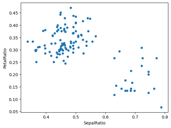
Since a function is passed in, the function is computed on the DataFrame being assigned to. Importantly, this is the DataFrame that’s been filtered to those rows with sepal length greater than 5. The filtering happens first, and then the ratio calculations. This is an example where we didn’t have a reference to the filtered DataFrame available.

The function signature for assign() is simply **kwargs. The keys are the column names for the new fields, and the values are either a value to be inserted (for example, a Series or NumPy array), or a function of one argument to be called on the DataFrame. A copy of the original DataFrame is returned, with the new values inserted.

The order of **kwargs is preserved. This allows for dependent assignment, where an expression later in **kwargs can refer to a column created earlier in the same assign().

dfa = pd.DataFrame({"A": [1, 2, 3], "B": [4, 5, 6]})

dfa.assign(C=lambda x: x["A"] + x["B"], D=lambda x: x["A"] + x["C"])

	A	B	C	D
0	1	4	5	6
1	2	5	7	9
2	3	6	9	12

In the second expression, x['C'] will refer to the newly created column, that’s equal to dfa['A'] + dfa['B'].

5.4.1.2.2.4. Indexing / selection

The basics of indexing are as follows:

Operation	Syntax	Result
Select column	df[col]	Series
Select row by label	df.loc[label]	Series
Select row by integer location	df.iloc[loc]	Series
Slice rows	df[5:10]	DataFrame
Select rows by boolean vector	df[bool_vec]	DataFrame

Row selection, for example, returns a Series whose index is the columns of the DataFrame:

df.loc["b"]

one            2.0
bar            2.0
flag         False
foo            bar
one_trunc      2.0
Name: b, dtype: object

from IPython.display import HTML

display(
    HTML(
        """


<link rel="stylesheet" href="https://ocademy-ai.github.io/machine-learning/_static/style.css">

<div class='full-width docutils' >
  <div class="admonition note pandastutor" name="html-admonition" style="margin-right:20%">
    <p class="admonition-title pandastutor">Let's visualize it! 🎥</p>
    <div class="pandastutor inner" style="height:730px;">
      <iframe frameborder="0" scrolling="no" src="https://pandastutor.com/vis.html#code=import%20pandas%20as%20pd%0Aimport%20io%0Aimport%20numpy%20as%20np%0Ad%20%3D%20%7B%0A%20%20%20%20%22one%22%3A%20pd.Series%28%5B1.0,%202.0,%203.0%5D,%20index%3D%5B%22a%22,%20%22b%22,%20%22c%22%5D%29,%0A%20%20%20%20%22two%22%3A%20pd.Series%28%5B1.0,%202.0,%203.0,%204.0%5D,%20index%3D%5B%22a%22,%20%22b%22,%20%22c%22,%20%22d%22%5D%29,%0A%7D%0Adf%20%3D%20pd.DataFrame%28d%29%0Adf%5B%22flag%22%5D%20%3D%20df%5B%22one%22%5D%20%3E%202%0Adel%20df%5B%22two%22%5D%0Adf%5B%22foo%22%5D%20%3D%20%22bar%22%0Adf%5B%22one_trunc%22%5D%20%3Ddf.insert%281,%20%22bar%22,%20df%5B%22one%22%5D%29%0Adf.loc%5B%22b%22%5D&d=2023-09-19&lang=py&v=v1"> </iframe>
    </div>
  </div>
</div>

"""
    )
)

Let's visualize it! 🎥

df.iloc[2]

one           3.0
bar           3.0
flag         True
foo           bar
one_trunc     NaN
Name: c, dtype: object

5.4.1.2.2.5. Data alignment and arithmetic

Data alignment between DataFrame objects automatically aligns on both the columns and the index (row labels)**. Again, the resulting object will have the union of the column and row labels.

df = pd.DataFrame(np.random.randn(10, 4), columns=["A", "B", "C", "D"])

df2 = pd.DataFrame(np.random.randn(7, 3), columns=["A", "B", "C"])

df + df2

	A	B	C	D
0	-1.065518	1.194950	0.030608	NaN
1	1.837983	0.316330	-2.104771	NaN
2	-1.381854	1.362421	1.120580	NaN
3	0.716434	-0.667963	-2.372925	NaN
4	1.813942	-2.189745	-1.778060	NaN
5	-0.680451	0.198311	-1.035426	NaN
6	0.070760	2.201920	1.783717	NaN
7	NaN	NaN	NaN	NaN
8	NaN	NaN	NaN	NaN
9	NaN	NaN	NaN	NaN

When doing an operation between DataFrame and Series, the default behavior is to align the Series index on the DataFrame columns, thus broadcasting row-wise. For example:

df - df.iloc[0]

	A	B	C	D
0	0.000000	0.000000	0.000000	0.000000
1	-0.153982	0.106456	-0.982637	-0.719556
2	-2.575348	0.616172	0.576169	-0.021143
3	-0.806753	-0.229733	-1.968249	-0.490483
4	0.546768	0.125705	-2.357085	-0.210174
5	0.595272	0.003298	-1.887417	1.366075
6	-0.927779	1.775162	0.936908	1.671263
7	-1.156538	0.646578	-0.663057	-0.767951
8	-1.152485	0.072190	-2.148250	-0.339899
9	-0.101024	-1.220136	-0.606941	0.116618

Arithmetic operations with scalars operate element-wise:

df * 5 + 2

	A	B	C	D
0	4.212800	2.056525	3.468874	2.697986
1	3.442890	2.588806	-1.444312	-0.899793
2	-8.663939	5.137387	6.349719	2.592272
3	0.179037	0.907857	-6.372371	0.245569
4	6.946641	2.685050	-8.316553	1.647115
5	7.189161	2.073015	-5.968211	9.528360
6	-0.426094	10.932335	8.153416	11.054301
7	-1.569888	5.289417	0.153589	-1.141768
8	-1.549626	2.417474	-7.272374	0.998492
9	3.707681	-4.044153	0.434168	3.281075

1 / df

	A	B	C	D
0	2.259580	88.456943	3.403968	7.163469
1	3.465268	8.491757	-1.451669	-1.724261
2	-0.468870	1.593683	1.149500	8.442063
3	-2.745800	-4.578157	-0.597202	-2.849926
4	1.010787	7.298739	-0.484658	-14.168931
5	0.963547	68.479290	-0.627493	0.664155
6	-2.060926	0.559764	0.812557	0.552224
7	-1.400604	1.520026	-2.707956	-1.591461
8	-1.408599	11.976801	-0.539236	-4.992471
9	2.927948	-0.827246	-3.193191	3.902973

df ** 4

	A	B	C	D
0	0.038361	1.633324e-08	0.007448	0.000380
1	0.006935	1.923135e-04	0.225180	0.113133
2	20.691434	1.550216e-01	0.572750	0.000197
3	0.017592	2.276341e-03	7.861654	0.015159
4	0.957991	3.523778e-04	18.124185	0.000025
5	1.160135	4.547398e-08	6.450052	5.139508
6	0.055431	1.018544e+01	2.293957	10.753247
7	0.259859	1.873250e-01	0.018597	0.155889
8	0.254010	4.860005e-05	11.827249	0.001610
9	0.013607	2.135315e+00	0.009618	0.004309

Boolean operators operate element-wise as well:

df1 = pd.DataFrame({"a": [1, 0, 1], "b": [0, 1, 1]}, dtype=bool)

df2 = pd.DataFrame({"a": [0, 1, 1], "b": [1, 1, 0]}, dtype=bool)

df1 & df2

	a	b
0	False	False
1	False	True
2	True	False

df1 | df2

	a	b
0	True	True
1	True	True
2	True	True

df1 ^ df2

	a	b
0	True	True
1	True	False
2	False	True

-df1

	a	b
0	False	True
1	True	False
2	False	False

5.4.1.2.2.6. Transposing

To transpose, access the T attribute or DataFrame.transpose(), similar to an ndarray:

df[:5].T

	0	1	2	3	4
A	0.442560	0.288578	-2.132788	-0.364193	0.989328
B	0.011305	0.117761	0.627477	-0.218429	0.137010
C	0.293775	-0.688862	0.869944	-1.674474	-2.063311
D	0.139597	-0.579959	0.118454	-0.350886	-0.070577

5.4.1.3. Data indexing and selection

The axis labeling information in Pandas objects serves many purposes:

• Identifies data (i.e. provides metadata) using known indicators, important for analysis, visualization, and interactive console display.

• Enables automatic and explicit data alignment.

• Allows intuitive getting and setting of subsets of the data set.

In this section, we will focus on the final point: namely, how to slice, dice, and generally get and set subsets of Pandas objects. The primary focus will be on Series and DataFrame as they have received more development attention in this area.

Note

The Python and NumPy indexing operators [] and attribute operator . provide quick and easy access to Pandas data structures across a wide range of use cases. This makes interactive work intuitive, as there’s little new to learn if you already know how to deal with Python dictionaries and NumPy arrays. However, since the type of the data to be accessed isn’t known in advance, directly using standard operators has some optimization limits. For production code, we recommended that you take advantage of the optimized Pandas data access methods exposed in this chapter.

Whether a copy or a reference is returned for a setting operation, may depend on the context. This is sometimes called chained assignment and should be avoided.

5.4.1.3.1. Different choices for indexing

Object selection has had a number of user-requested additions in order to support more explicit location-based indexing. Pandas now supports three types of multi-axis indexing.

• .loc is primarily label based, but may also be used with a boolean array. .loc will raise KeyError when the items are not found. Allowed inputs are:

  • A single label, e.g. 5 or 'a' (Note that 5 is interpreted as a label of the index. This use is not an integer position along the index.).

  • A list or array of labels ['a', 'b', 'c'].

  • A slice object with labels 'a':'f' (Note that contrary to usual Python slices, both the start and the stop are included, when present in the index!)

  • A boolean array (any NA values will be treated as False).

  • A callable function with one argument (the calling Series or DataFrame) and that returns valid output for indexing (one of the above).

• .iloc is primarily integer position based (from 0 to length-1 of the axis), but may also be used with a boolean array. .iloc will raise IndexError if a requested indexer is out-of-bounds, except slice indexers which allow out-of-bounds indexing. (this conforms with Python/NumPy slice semantics). Allowed inputs are:

  • An integer e.g. 5.

  • A list or array of integers [4, 3, 0].

  • A slice object with ints 1:7.

  • A boolean array (any NA values will be treated as False).

  • A callable function with one argument (the calling Series or DataFrame) that returns valid output for indexing (one of the above).

• .loc, .iloc, and also [] indexing can accept a callable as indexer.

Getting values from an object with multi-axes selection uses the following notation (using .loc as an example, but the following applies to .iloc as well). Any of the axes accessors may be the null slice :. Axes left out of the specification are assumed to be :, e.g. p.loc['a'] is equivalent to p.loc['a', :].

Object Type	Indexers
Series	s.loc[indexer]
DataFrame	df.loc[row_indexer, column_indexer]

5.4.1.3.2. Basics

As mentioned when introducing the data structures in the last section, the primary function of indexing with [] (a.k.a. __getitem__ for those familiar with implementing class behavior in Python) is selecting out lower-dimensional slices. The following table shows return type values when indexing Pandas objects with []:

Object Type	Selection	Return Value Type
Series	series[label]	scalar value
DataFrame	frame[colname]	Series corresponding to colname

Here we construct a simple time series data set to use for illustrating the indexing functionality:

dates = pd.date_range('1/1/2000', periods=8)
df = pd.DataFrame(np.random.randn(8, 4),
                  index=dates, columns=['A', 'B', 'C', 'D'])
df

	A	B	C	D
2000-01-01	0.711418	0.603204	-0.417841	1.391724
2000-01-02	-0.744106	0.862873	1.216255	-1.282529
2000-01-03	-1.373171	1.581176	0.828784	-2.048825
2000-01-04	-0.588767	-2.798199	-0.018800	0.130053
2000-01-05	1.251814	0.068020	0.373987	-0.041853
2000-01-06	-0.377347	0.654981	0.059024	0.507564
2000-01-07	0.111746	0.016025	-1.023215	-0.677410
2000-01-08	1.409014	0.481835	-0.756125	2.236706

Note

None of the indexing functionality is time series specific unless specifically stated.

Thus, as per above, we have the most basic indexing using []:

s = df['A']

s[dates[5]]

-0.3773466384496966

You can pass a list of columns to [] to select columns in that order. If a column is not contained in the DataFrame, an exception will be raised. Multiple columns can also be set in this manner:

df

	A	B	C	D
2000-01-01	0.711418	0.603204	-0.417841	1.391724
2000-01-02	-0.744106	0.862873	1.216255	-1.282529
2000-01-03	-1.373171	1.581176	0.828784	-2.048825
2000-01-04	-0.588767	-2.798199	-0.018800	0.130053
2000-01-05	1.251814	0.068020	0.373987	-0.041853
2000-01-06	-0.377347	0.654981	0.059024	0.507564
2000-01-07	0.111746	0.016025	-1.023215	-0.677410
2000-01-08	1.409014	0.481835	-0.756125	2.236706

df[['B', 'A']] = df[['A', 'B']]
df

	A	B	C	D
2000-01-01	0.603204	0.711418	-0.417841	1.391724
2000-01-02	0.862873	-0.744106	1.216255	-1.282529
2000-01-03	1.581176	-1.373171	0.828784	-2.048825
2000-01-04	-2.798199	-0.588767	-0.018800	0.130053
2000-01-05	0.068020	1.251814	0.373987	-0.041853
2000-01-06	0.654981	-0.377347	0.059024	0.507564
2000-01-07	0.016025	0.111746	-1.023215	-0.677410
2000-01-08	0.481835	1.409014	-0.756125	2.236706

You may find this useful for applying a transform (in-place) to a subset of the columns.

Pandas aligns all AXES when setting Series and DataFrame from .loc, and .iloc.

This will not modify df because the column alignment is before value assignment.

df[['A', 'B']]

	A	B
2000-01-01	0.603204	0.711418
2000-01-02	0.862873	-0.744106
2000-01-03	1.581176	-1.373171
2000-01-04	-2.798199	-0.588767
2000-01-05	0.068020	1.251814
2000-01-06	0.654981	-0.377347
2000-01-07	0.016025	0.111746
2000-01-08	0.481835	1.409014

df.loc[:, ['B', 'A']] = df[['A', 'B']]
df[['A', 'B']]

	A	B
2000-01-01	0.603204	0.711418
2000-01-02	0.862873	-0.744106
2000-01-03	1.581176	-1.373171
2000-01-04	-2.798199	-0.588767
2000-01-05	0.068020	1.251814
2000-01-06	0.654981	-0.377347
2000-01-07	0.016025	0.111746
2000-01-08	0.481835	1.409014

The correct way to swap column values is by using raw values:

df.loc[:, ['B', 'A']] = df[['A', 'B']].to_numpy()
df[['A', 'B']]

	A	B
2000-01-01	0.711418	0.603204
2000-01-02	-0.744106	0.862873
2000-01-03	-1.373171	1.581176
2000-01-04	-0.588767	-2.798199
2000-01-05	1.251814	0.068020
2000-01-06	-0.377347	0.654981
2000-01-07	0.111746	0.016025
2000-01-08	1.409014	0.481835

5.4.1.3.3. Attribute access

You may access an index on a Series or column on a DataFrame directly as an attribute:

sa = pd.Series([1, 2, 3], index=list('abc'))
dfa = df.copy()

sa.b

2

dfa.A

2000-01-01    0.711418
2000-01-02   -0.744106
2000-01-03   -1.373171
2000-01-04   -0.588767
2000-01-05    1.251814
2000-01-06   -0.377347
2000-01-07    0.111746
2000-01-08    1.409014
Freq: D, Name: A, dtype: float64

sa.a = 5
sa

a    5
b    2
c    3
dtype: int64

dfa.A = list(range(len(dfa.index)))  # ok if A already exists
dfa

	A	B	C	D
2000-01-01	0	0.603204	-0.417841	1.391724
2000-01-02	1	0.862873	1.216255	-1.282529
2000-01-03	2	1.581176	0.828784	-2.048825
2000-01-04	3	-2.798199	-0.018800	0.130053
2000-01-05	4	0.068020	0.373987	-0.041853
2000-01-06	5	0.654981	0.059024	0.507564
2000-01-07	6	0.016025	-1.023215	-0.677410
2000-01-08	7	0.481835	-0.756125	2.236706

dfa['A'] = list(range(len(dfa.index)))  # use this form to create a new column
dfa

	A	B	C	D
2000-01-01	0	0.603204	-0.417841	1.391724
2000-01-02	1	0.862873	1.216255	-1.282529
2000-01-03	2	1.581176	0.828784	-2.048825
2000-01-04	3	-2.798199	-0.018800	0.130053
2000-01-05	4	0.068020	0.373987	-0.041853
2000-01-06	5	0.654981	0.059024	0.507564
2000-01-07	6	0.016025	-1.023215	-0.677410
2000-01-08	7	0.481835	-0.756125	2.236706

• You can use this access only if the index element is a valid Python identifier, e.g. s.1 is not allowed. See here for an explanation of valid identifiers.

• The attribute will not be available if it conflicts with an existing method name, e.g. s.min is not allowed, but s[‘min’] is possible.

• Similarly, the attribute will not be available if it conflicts with any of the following list: index, major_axis, minor_axis, items.

• In any of these cases, standard indexing will still work, e.g. s[‘1’], s[‘min’], and s[‘index’] will access the corresponding element or column.

If you are using the IPython environment, you may also use tab-completion to see these accessible attributes.

You can also assign a dict to a row of a DataFrame:

x = pd.DataFrame({'x': [1, 2, 3], 'y': [3, 4, 5]})
x.iloc[1] = {'x': 9, 'y': 99}
x

	x	y
0	1	3
1	9	99
2	3	5

You can use attribute access to modify an existing element of a Series or column of a DataFrame, but be careful; if you try to use attribute access to create a new column, it creates a new attribute rather than a new column. In 0.21.0 and later, this will raise a UserWarning:

df = pd.DataFrame({'one': [1., 2., 3.]})
df.two = [4, 5, 6]

/tmp/ipykernel_2921/269534380.py:2: UserWarning: Pandas doesn't allow columns to be created via a new attribute name - see https://pandas.pydata.org/pandas-docs/stable/indexing.html#attribute-access
  df.two = [4, 5, 6]

df

	one
0	1.0
1	2.0
2	3.0

5.4.1.3.4. Slicing ranges

For now, we explain the semantics of slicing using the [] operator.

With Series, the syntax works exactly as with an ndarray, returning a slice of the values and the corresponding labels:

s

2000-01-01    0.711418
2000-01-02   -0.744106
2000-01-03   -1.373171
2000-01-04   -0.588767
2000-01-05    1.251814
2000-01-06   -0.377347
2000-01-07    0.111746
2000-01-08    1.409014
Freq: D, Name: A, dtype: float64

s[:5]

2000-01-01    0.711418
2000-01-02   -0.744106
2000-01-03   -1.373171
2000-01-04   -0.588767
2000-01-05    1.251814
Freq: D, Name: A, dtype: float64

s[::2]

2000-01-01    0.711418
2000-01-03   -1.373171
2000-01-05    1.251814
2000-01-07    0.111746
Freq: 2D, Name: A, dtype: float64

s[::-1]

2000-01-08    1.409014
2000-01-07    0.111746
2000-01-06   -0.377347
2000-01-05    1.251814
2000-01-04   -0.588767
2000-01-03   -1.373171
2000-01-02   -0.744106
2000-01-01    0.711418
Freq: -1D, Name: A, dtype: float64

Note that setting works as well:

s2 = s.copy()
s2[:5] = 0
s2

2000-01-01    0.000000
2000-01-02    0.000000
2000-01-03    0.000000
2000-01-04    0.000000
2000-01-05    0.000000
2000-01-06   -0.377347
2000-01-07    0.111746
2000-01-08    1.409014
Freq: D, Name: A, dtype: float64

With DataFrame, slicing inside of [] slices the rows. This is provided largely as a convenience since it is such a common operation.

df[:3]

	one
0	1.0
1	2.0
2	3.0

df[::-1]

	one
2	3.0
1	2.0
0	1.0

5.4.1.4. Acknowledgments

Thanks for Pandas user guide. It contributes the majority of the content in this chapter.