# Install the necessary dependencies

import os
import sys
!{sys.executable} -m pip install --quiet seaborn pandas scikit-learn numpy matplotlib jupyterlab_myst ipython

15. Getting started with ensemble learning

In previous sections, we explored different classification algorithms as well as techniques that can be used to properly validate and evaluate the quality of your models.

Now, suppose that we have chosen the best possible model for a particular problem and are struggling to further improve its accuracy. In this case, we would need to apply some more advanced machine learning techniques that are collectively referred to as ensembles.

An ensemble is a set of elements that collectively contribute to a whole. A familiar example is a musical ensemble, which blends the sounds of several musical instruments to create harmony, or architectural ensembles, which are a set of buildings designed as a unit. In ensembles, the (whole) harmonious outcome is more important than the performance of any individual part.

Ensembles

Condorcet’s jury theorem (1784) is about an ensemble in some sense. It states that, if each member of the jury makes an independent judgment and the probability of the correct decision by each juror is more than 0.5, then the probability of the correct decision by the whole jury increases with the total number of jurors and tends to one. On the other hand, if the probability of being right is less than 0.5 for each juror, then the probability of the correct decision by the whole jury decreases with the number of jurors and tends to zero.

Let’s write an analytic expression for this theorem:

• \(\large N\) is the total number of jurors;

• \(\large m\) is a minimal number of jurors that would make a majority, that is \(\large m = floor(N/2) + 1\);

• \(\large {N \choose i}\) is the number of \(\large i\)-combinations from a set with \(\large N\) elements.

• \(\large p\) is the probability of the correct decision by a juror;

• \(\large \mu\) is the probability of the correct decision by the whole jury.

Then:

\[ \large \mu = \sum_{i=m}^{N}{N\choose i}p^i(1-p)^{N-i} \]

It can be seen that if \(\large p > 0.5\), then \(\large \mu > p\). In addition, if \(\large N \rightarrow \infty \), then \(\large \mu \rightarrow 1\).

\(~~~~~~~\)… whenever we are faced with making a decision that has some important consequence, we often seek the opinions of different “experts”

\(~~~~~~\) to help us that decision …

\(~~~~~~~~~~~~~~~~~~~~~~~~~~~~~~~~~~~~~~~~~~~~~~~~~~~~~~~~~~~~~~~~~~~~~~~~~~~~~~~~~~~~~~~~~~~~~~~~~~~~~~~~~~~~~~~~~~~~~~~~~~~~~~~~~~~~~~~~~~~~\) — Page 2, Ensemble Machine Learning, 2012.

Let’s look at another example of ensembles: an observation known as Wisdom of the crowd. In 1906, Francis Galton visited a country fair in Plymouth where he saw a contest being held for farmers. 800 participants tried to estimate the weight of a slaughtered bull. The real weight of the bull was 1198 pounds. Although none of the farmers could guess the exact weight of the animal, the average of their predictions was 1197 pounds.

A similar idea for error reduction was also adopted in the field of Ensemble Learning which is called voting.

The video below will show you what is Ensemble Learning and introduce several methods of Ensemble Learning.

from IPython.display import HTML
display(HTML("""
<div class="yt-container">
   <iframe src="https://www.youtube.com/embed/r00tBoV1lHw?si=QaFvP7NJ6s3A_Dca" allowfullscreen></iframe>
</div>
"""))

Intuition for classification ensembles

A model that learns how to classify points in effect draws lines in the feature space to separate examples. We can sample points in the feature space in a grid and get a map of how the model thinks the feature space should be by each class label. The separation of examples in the feature space by the model is called the decision boundary and a plot of the grid or map of how the model classifies points in the feature space is called a decision boundary plot. Now consider an ensemble where each model has a different mapping of inputs to outputs. In effect, each model has a different decision boundary or different idea of how to split up in the feature space by class label. Each model will draw the lines differently and make different errors. When we combine the predictions from these multiple different models, we are in effect averaging the decision boundaries. We are defining a new decision boundary that attempts to learn from all the different views on the feature space learned by contributing members.

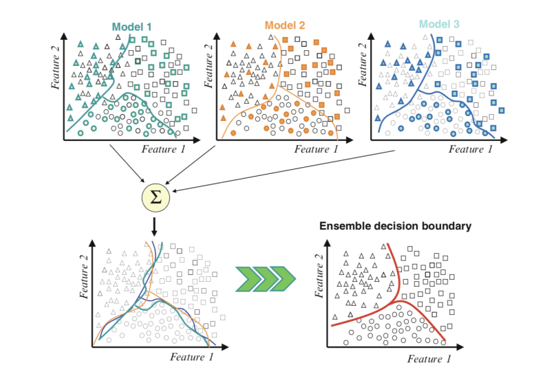
Fig. 15.1 Example of Combining Decision Boundaries Using an Ensemble. Taken from Ensemble Machine Learning, 2012

We can see the contributing members along the top, each with different decision boundaries in the feature space. Then the bottom-left draws all of the decision boundaries on the same plot showing how they differ and make different errors. Finally, we can combine these boundaries to in-effect create a new generalized decision boundary in the bottom-right that better captures the true but unknown division of the feature space, resulting in better predictive performance.

We have learned what ensemble learning is, and in the next chapter, we will learn some specific algorithms for ensemble learning

15.1. Acknowledgments

Thanks to the book Ensemble Machine Learning: Methods and Applications 2012th Edition by Cha Zhang (Editor), Yunqian Ma (Editor). They inspire the majority of the content in this chapter.