42.68. Decision Trees - Intro and Regression#

Decision Trees are supervised machine learning algorithms that are used for both regression and classification tasks. Trees are powerful algorithms that can handle complex datasets.

Here are 7 interesting facts about decision trees:

They do not need the numerical input data to be scaled. Whatever the numerical values are, decision trees don’t care.
Decision trees handle categorical features in the raw text format (Scikit-Learn doesn’t support this, TensorFlow’s trees implementation does).
Different to other complex learning algorithms, the results of decision trees can be interpreted. It’s fair to say that decision trees are not blackbox type models.
While most models will suffer from missing values, decision trees are okay with them.
Trees can handle imbalanced datasets. You will only have to adjust the weights of the classes.
Trees can provide the feature importances or how much each feature contributed to the model training results.
Trees are the basic building blocks of ensemble methods such as random forests and gradient boosting machines.

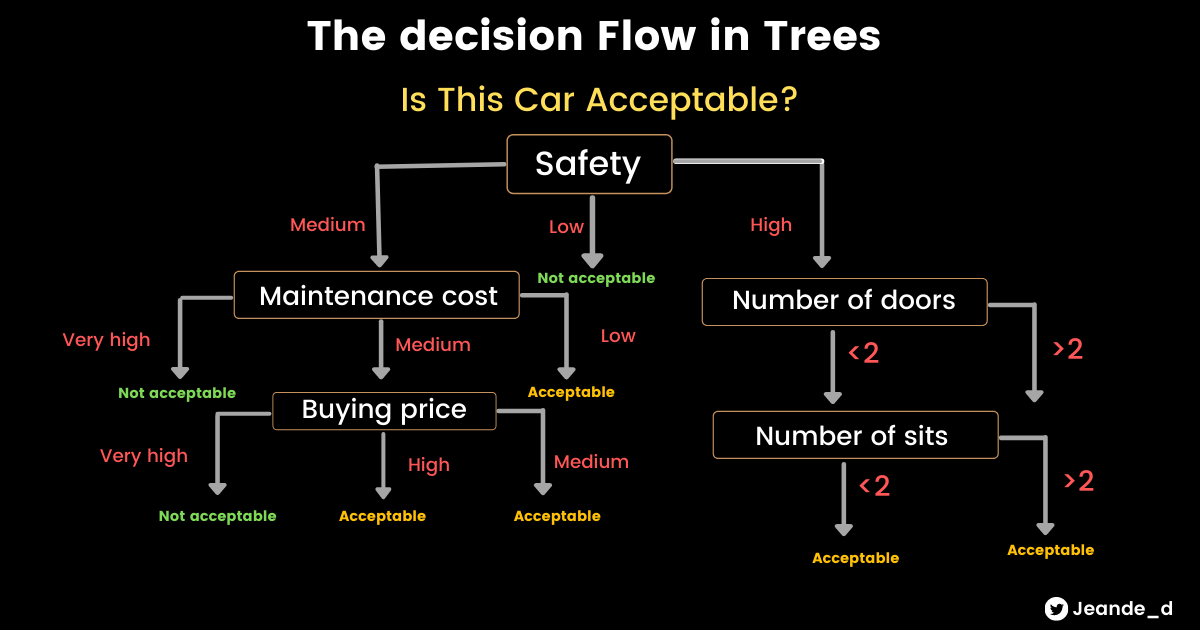
The way decision trees works is like the series of if/else questions. Let’s say that you want to make a decision of the car to buy. In order to get the right car to buy, you could go on and evaluate the level of the safety, the number of sits and doors by asking series of if like questions.

Here is the structure of the decision trees.

Decision Trees.png

A well-known downside of decision trees is that they tend to overfit the data easily(pretty much assumed they will always overfit at first). One way to overcome overfitting is to reduce the maximum depth of the decision tree (refered to as max_depthhyperparameter) in decision trees. We will see other techniques to avoid overfitting.

To motivate the superpower of decision trees, let’s use it for a regression task where instead of predicting class, we are predicting a continous value. In the next lab, we will use them for classification.

42.68.1. Decision Trees for Regression#

42.68.1.1. Contents#

[1 - Imports]
[2 - Loading the data]
[3 - Exploratory Analysis]
[4 - Preprocessing the data]
[5 - Training Decision Trees]
[6 - Evaluating Decision Trees]
[7 - Improving Decision Trees]

42.68.2. 1 - Imports#

import numpy as np
import pandas as pd
import seaborn as sns
import sklearn
import matplotlib.pyplot as plt
%matplotlib inline

42.68.3. 2 - Loading the data#

In this regression task with decision trees, we will use the Machine CPU (Central Processing Unit) data which is avilable at OpenML. We will load it with Sklearn fetch_openml function.

If you are reading this, it’s very likely that you know CPU or you have once(or many times) thought about it when you were buying your computer. In this notebook, we will predict the relative performance of the CPU given the following data:

MYCT: machine cycle time in nanoseconds (integer)
MMIN: minimum main memory in kilobytes (integer)
MMAX: maximum main memory in kilobytes (integer)
CACH: cache memory in kilobytes (integer)
CHMIN: minimum channels in units (integer)
CHMAX: maximum channels in units (integer)
PRP: published relative performance (integer) (target variable)

# Let's hide warnings

import warnings
warnings.filterwarnings('ignore')

from sklearn.datasets import fetch_openml

machine_cpu = fetch_openml(name='machine_cpu')

type(machine_cpu)

sklearn.utils._bunch.Bunch

machine_cpu.data.shape

(209, 6)

print(machine_cpu.DESCR)

**Author**:   
**Source**: Unknown -   
**Please cite**:   

The problem concerns Relative CPU Performance Data. More information can be obtained in the UCI Machine
 Learning repository (http://www.ics.uci.edu/~mlearn/MLSummary.html).
 The used attributes are :
 MYCT: machine cycle time in nanoseconds (integer)
 MMIN: minimum main memory in kilobytes (integer)
 MMAX: maximum main memory in kilobytes (integer)
 CACH: cache memory in kilobytes (integer)
 CHMIN: minimum channels in units (integer)
 CHMAX: maximum channels in units (integer)
 PRP: published relative performance (integer) (target variable)
 
 Original source: UCI machine learning repository. 
 Source: collection of regression datasets by Luis Torgo (ltorgo@ncc.up.pt) at
 http://www.ncc.up.pt/~ltorgo/Regression/DataSets.html
 Characteristics: 209 cases; 6 continuous variables

Downloaded from openml.org.

# Displaying feature names

machine_cpu.feature_names

['MYCT', 'MMIN', 'MMAX', 'CACH', 'CHMIN', 'CHMAX']

# Getting the whole dataframe

machine_cpu.frame

	MYCT	MMIN	MMAX	CACH	CHMIN	CHMAX	class
0	125.0	256.0	6000.0	256.0	16.0	128.0	198.0
1	29.0	8000.0	32000.0	32.0	8.0	32.0	269.0
2	29.0	8000.0	32000.0	32.0	8.0	32.0	220.0
3	29.0	8000.0	32000.0	32.0	8.0	32.0	172.0
4	29.0	8000.0	16000.0	32.0	8.0	16.0	132.0
...	...	...	...	...	...	...	...
204	124.0	1000.0	8000.0	0.0	1.0	8.0	42.0
205	98.0	1000.0	8000.0	32.0	2.0	8.0	46.0
206	125.0	2000.0	8000.0	0.0	2.0	14.0	52.0
207	480.0	512.0	8000.0	32.0	0.0	0.0	67.0
208	480.0	1000.0	4000.0	0.0	0.0	0.0	45.0

209 rows × 7 columns

Now, let’s get the data and labels.

machine_data = machine_cpu.data
machine_labels = machine_cpu.target

type(machine_data)

pandas.core.frame.DataFrame

type(machine_labels)

pandas.core.series.Series

42.68.4. 3 - Exploratory Analysis#

Before doing exploratory analysis, let’s get the training and test data.

from sklearn.model_selection import train_test_split

X_train, X_test, y_train, y_test = train_test_split(machine_data,machine_labels, test_size=0.2,random_state=20)

print('The size of training data is: {} \nThe size of testing data is: {}'.format(len(X_train), len(X_test)))

The size of training data is: 167 
The size of testing data is: 42

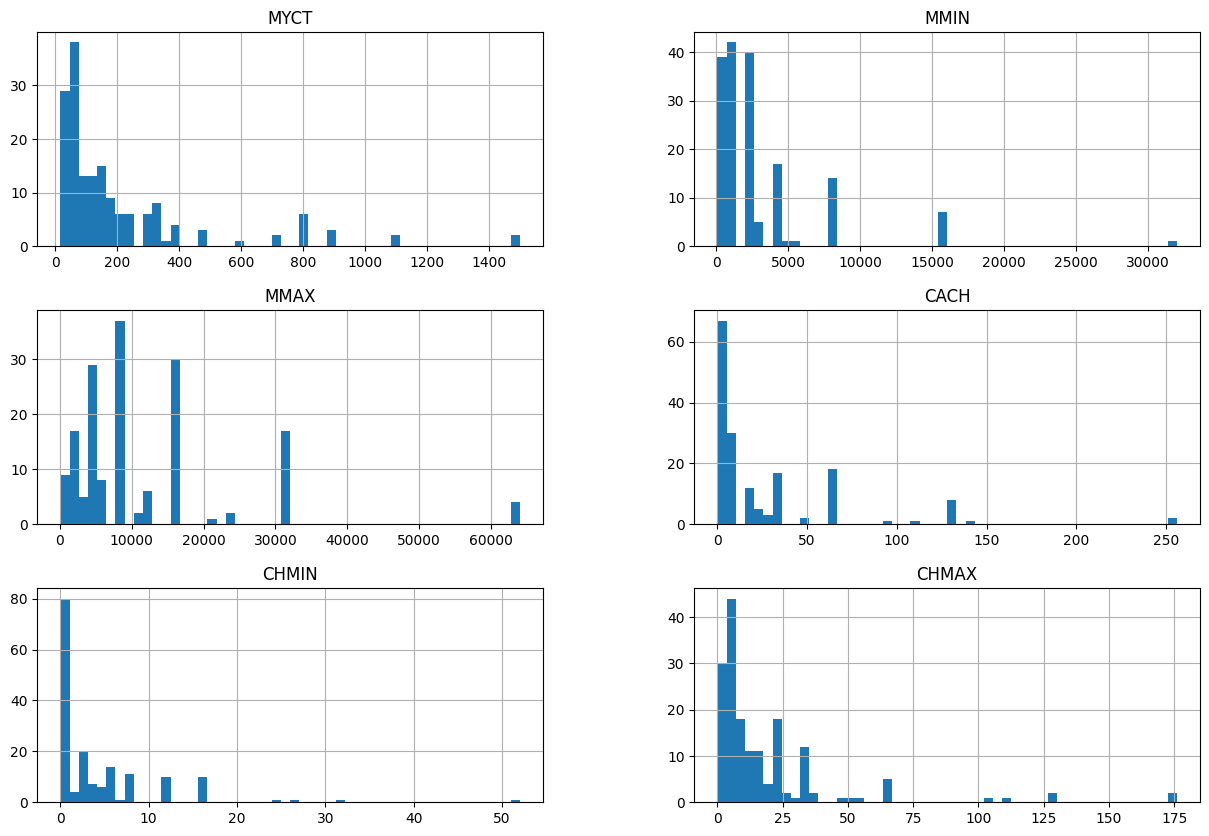
Let’s visualize the histograms of all numeric features.

X_train.hist(bins=50, figsize=(15,10))
plt.show()

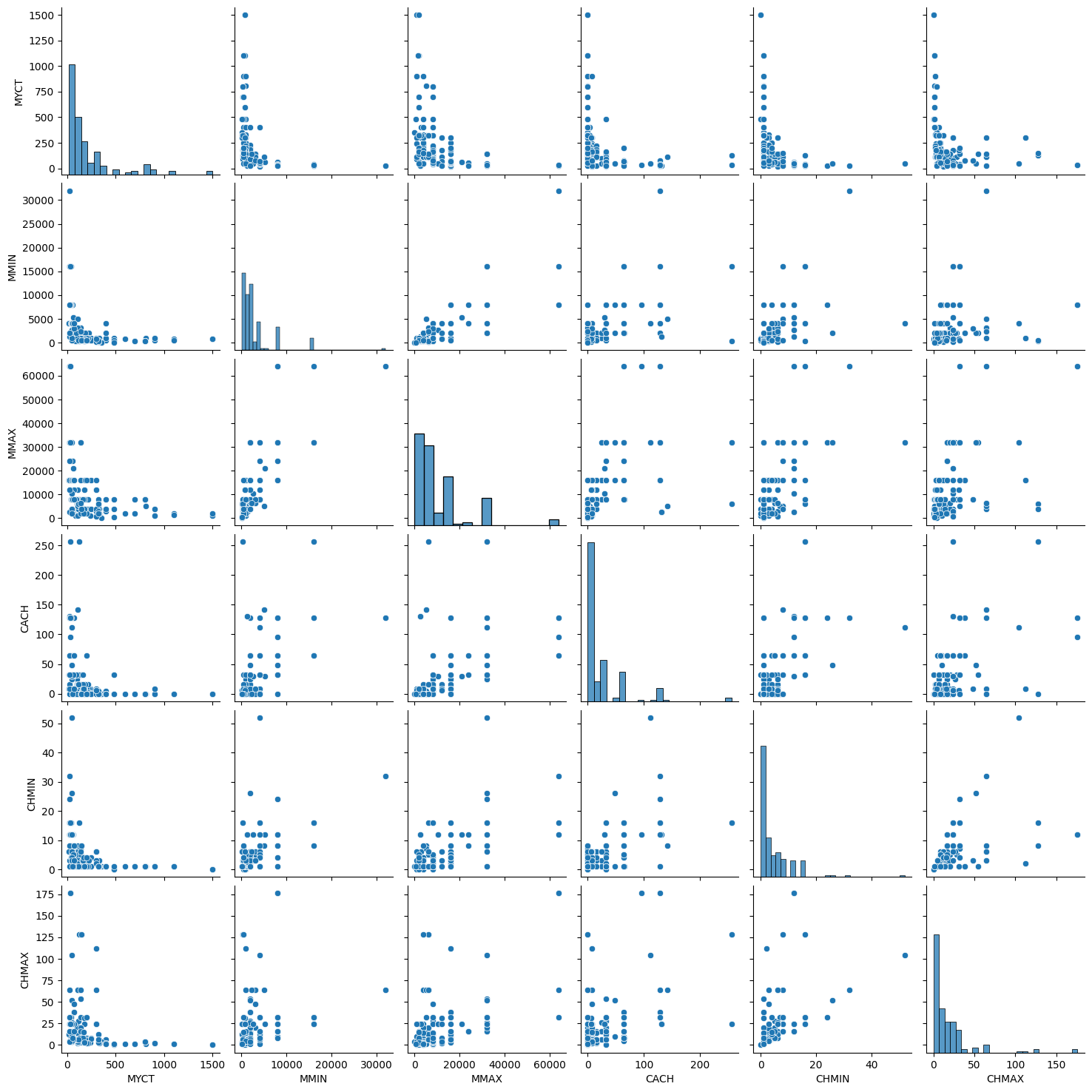
../../../_images/decision_trees_for_regression_22_0.png

Or we can quickly use sns.pairplot() to look into the data.

sns.pairplot(X_train)

<seaborn.axisgrid.PairGrid at 0x227c78bf790>

../../../_images/decision_trees_for_regression_24_1.png

# Checking summary stats

X_train.describe()

	MYCT	MMIN	MMAX	CACH	CHMIN	CHMAX
count	167.000000	167.000000	167.000000	167.000000	167.000000	167.000000
mean	207.958084	2900.826347	11761.161677	26.071856	4.760479	18.616766
std	266.772823	4165.950964	12108.332354	42.410014	6.487439	27.489919
min	17.000000	64.000000	64.000000	0.000000	0.000000	0.000000
25%	50.000000	768.000000	4000.000000	0.000000	1.000000	5.000000
50%	110.000000	2000.000000	8000.000000	8.000000	2.000000	8.000000
75%	232.500000	3100.000000	16000.000000	32.000000	6.000000	24.000000
max	1500.000000	32000.000000	64000.000000	256.000000	52.000000	176.000000

# Checking missing values

X_train.isnull().sum()

MYCT     0
MMIN     0
MMAX     0
CACH     0
CHMIN    0
CHMAX    0
dtype: int64

We don’t have any missing values.

42.68.5. 4 - Data Preprocessing#

It is here that we prepare the data to be in the proper format for the machine learning model.

Decision trees don’t care if the features are scaled or not. Let’s set up a pipeline to scale features, and we will use it to verify that notion.

from sklearn.preprocessing import StandardScaler
from sklearn.pipeline import Pipeline

scale_pipe = Pipeline([
    ('scaler', StandardScaler())
    
])

X_train_scaled = scale_pipe.fit_transform(X_train)

42.68.6. 5 - Training Decision Tree Regressor#

from sklearn.tree import DecisionTreeRegressor

tree_reg = DecisionTreeRegressor()

tree_reg.fit(X_train, y_train)

DecisionTreeRegressor()

In a Jupyter environment, please rerun this cell to show the HTML representation or trust the notebook.
On GitHub, the HTML representation is unable to render, please try loading this page with nbviewer.org.

Let’s train the same model on the scaled data.

tree_reg_scaled = DecisionTreeRegressor()

tree_reg_scaled.fit(X_train_scaled, y_train)

DecisionTreeRegressor()

42.68.7. 6 - Evaluating Decision Trees#

Let’s first check the root mean squarred errr on the training. It is not advised to evaluate the model on the test data since we haven’t improved it yet. I will make a function to make it easier and to avoid repetitions.

from sklearn.metrics import mean_squared_error

def predict(input_data,model,labels):
    """
    Take the input data, model and labels and return predictions
    
    """
    
    preds = model.predict(input_data)
    mse = mean_squared_error(labels,preds)
    rmse = np.sqrt(mse)
    rmse
    
    return rmse

predict(X_train, tree_reg, y_train)

9.724590719956222

And when the training data is scaled…

predict(X_train_scaled, tree_reg_scaled, y_train)

9.724590719956222

As you can see, there is no difference at all. So in your future projects using decision trees, whether you scale the data or not, your predictions will not be affected.

But don’t do this…

predict(X_train_scaled, tree_reg, y_train)

201.6303904952264

If you can inspect the parameters that I passed in predict function above, there are scaled data, model trained on unscaled data, and labels(y_train). As you may have guessed, that is a complete mismatch which led to poor results. If you trained a model on scaled data, the data that you predict the model on should be scaled in the same way too.

Let’s try to improve the model.

42.68.8. 7 - Improving Decision Trees#

tree_reg.get_params()

{'ccp_alpha': 0.0,
 'criterion': 'squared_error',
 'max_depth': None,
 'max_features': None,
 'max_leaf_nodes': None,
 'min_impurity_decrease': 0.0,
 'min_samples_leaf': 1,
 'min_samples_split': 2,
 'min_weight_fraction_leaf': 0.0,
 'random_state': None,
 'splitter': 'best'}

We have seen that one way to improve the decision tree model is to find the right number of max_depth and some other few parameters. Let’s use GridSearch to find best hyperparameters. Note that this may end up overfitting because we have a small dataset. But since we are doing this for learning purpose (you can adapt it to your problem), let’s do it.

from sklearn.model_selection import GridSearchCV

params_grid = {'max_leaf_nodes': list(range(0, 10)), 'min_samples_split': [0,1,2, 3, 4], 
              'max_depth':[None,0,1,2,3]}

#refit is true by default. The best estimator is trained on the whole dataset 

grid_search = GridSearchCV(DecisionTreeRegressor(random_state=42), params_grid, verbose=1, cv=3, refit=True)

grid_search.fit(X_train, y_train)

Fitting 3 folds for each of 250 candidates, totalling 750 fits

GridSearchCV(cv=3, estimator=DecisionTreeRegressor(random_state=42),
             param_grid={'max_depth': [None, 0, 1, 2, 3],
                         'max_leaf_nodes': [0, 1, 2, 3, 4, 5, 6, 7, 8, 9],
                         'min_samples_split': [0, 1, 2, 3, 4]},
             verbose=1)

grid_search.best_params_

{'max_depth': None, 'max_leaf_nodes': 9, 'min_samples_split': 4}

grid_search.best_estimator_

DecisionTreeRegressor(max_leaf_nodes=9, min_samples_split=4, random_state=42)

tree_best = grid_search.best_estimator_

Let’s make prediction on the training data again

predict(X_train, tree_best, y_train)

34.999530266023044

Like we said, we overfitted. The RMSE on our small dataset was pretty enough (and you probably would not use decision trees for small data like this we are using).

Finally we can evaluate the model on the test set. Let’s use the orginal model.

predict(X_test, tree_reg, y_test)

43.10928802805393

Clearly, the model overfitted and the improvements we tried didn’t improve anything. This is not an issue of the model or our approach to improve the model. Decision trees are complex models for the data we have.

This is the end of the notebook. We have learned the fundamental idea behind the decision trees, and used it to predict the CPU performance. In the next lab, we will use it for classification task and we will use a real world dataset so that we can practically improve the decision trees model.

42.68.9. Acknowledgments#

Thanks to Jake VanderPlas for creating the open-source course Python Data Science Handbook . It inspires the majority of the content in this chapter.

Ocademy Open Machine Learning Book

Decision Trees - Intro and Regression

Contents