Unsupervised learning
Contents
# Install the necessary dependencies

import os
import sys
!{sys.executable} -m pip install --quiet pandas scikit-learn numpy matplotlib jupyterlab_myst ipython
17. Unsupervised learning#
First, let’s import a few common modules, ensure MatplotLib plots figures inline and prepare a function to save the figures. We also check that Python 3.5 or later is installed (although Python 2.x may work, it is deprecated so we strongly recommend you use Python 3 instead), as well as Scikit-Learn ≥0.20.
# Python ≥3.5 is required
import sys
assert sys.version_info >= (3, 5)

# Scikit-Learn ≥0.20 is required
import sklearn
assert sklearn.__version__ >= "0.20"

# Common imports
import numpy as np
import os

# to make this notebook's output stable across runs
np.random.seed(42)

# To plot pretty figures
%matplotlib inline
import matplotlib as mpl
import matplotlib.pyplot as plt

import warnings
warnings.filterwarnings("ignore", category=FutureWarning, module="sklearn")

mpl.rc('axes', labelsize=14)
mpl.rc('xtick', labelsize=12)
mpl.rc('ytick', labelsize=12)

# Where to save the figures
PROJECT_ROOT_DIR = "."
CHAPTER_ID = "unsupervised_learning"
IMAGES_PATH = os.path.join(PROJECT_ROOT_DIR, "images", CHAPTER_ID)
os.makedirs(IMAGES_PATH, exist_ok=True)

def save_fig(fig_id, tight_layout=True, fig_extension="png", resolution=300):
    path = os.path.join(IMAGES_PATH, fig_id + "." + fig_extension)
    print("Saving figure", fig_id)
    if tight_layout:
        plt.tight_layout()
    plt.savefig(path, format=fig_extension, dpi=resolution)
17.1. K-Means#
from IPython.display import HTML
display(HTML("""
<p style="text-align: center;">
<iframe src="https://static-1300131294.cos.ap-shanghai.myqcloud.com/html/k-means-demo/k-means.html" width="105%" height="800px;"
style="border:none;" scrolling="auto"></iframe>
A demo of linear-regression. <a
href="http://alekseynp.com/viz/k-means.html"> [source]</a>
</p>
"""))
A demo of linear-regression. [source]
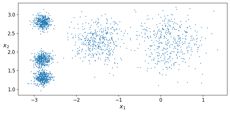
Let’s start by generating some blobs:
from sklearn.datasets import make_blobs
blob_centers = np.array(
    [[ 0.2,  2.3],
     [-1.5 ,  2.3],
     [-2.8,  1.8],
     [-2.8,  2.8],
     [-2.8,  1.3]])
blob_std = np.array([0.4, 0.3, 0.1, 0.1, 0.1])
X, y = make_blobs(n_samples=2000, centers=blob_centers,
                  cluster_std=blob_std, random_state=7)
Now let’s plot them:
def plot_clusters(X, y=None):
    plt.scatter(X[:, 0], X[:, 1], c=y, s=1)
    plt.xlabel("$x_1$", fontsize=14)
    plt.ylabel("$x_2$", fontsize=14, rotation=0)
plt.figure(figsize=(8, 4))
plot_clusters(X)
save_fig("blobs_plot")
plt.show()
Saving figure blobs_plot
Let’s train a K-Means clusterer on this dataset. It will try to find each blob’s center and assign each instance to the closest blob:
from sklearn.cluster import KMeans
k = 5
kmeans = KMeans(n_clusters=k, random_state=42)
y_pred = kmeans.fit_predict(X)
Each instance was assigned to one of the 5 clusters:
y_pred
array([4, 0, 1, ..., 2, 1, 0], dtype=int32)
y_pred is kmeans.labels_
True
And the following 5 centroids (i.e., cluster centers) were estimated:
kmeans.cluster_centers_
array([[-2.80389616,  1.80117999],
       [ 0.20876306,  2.25551336],
       [-2.79290307,  2.79641063],
       [-1.46679593,  2.28585348],
       [-2.80037642,  1.30082566]])
Note that the KMeans instance preserves the labels of the instances it was trained on. Somewhat confusingly, in this context, the label of an instance is the index of the cluster that instance gets assigned to:
kmeans.labels_
array([4, 0, 1, ..., 2, 1, 0], dtype=int32)
Of course, we can predict the labels of new instances:
X_new = np.array([[0, 2], [3, 2], [-3, 3], [-3, 2.5]])
kmeans.predict(X_new)
array([1, 1, 2, 2], dtype=int32)
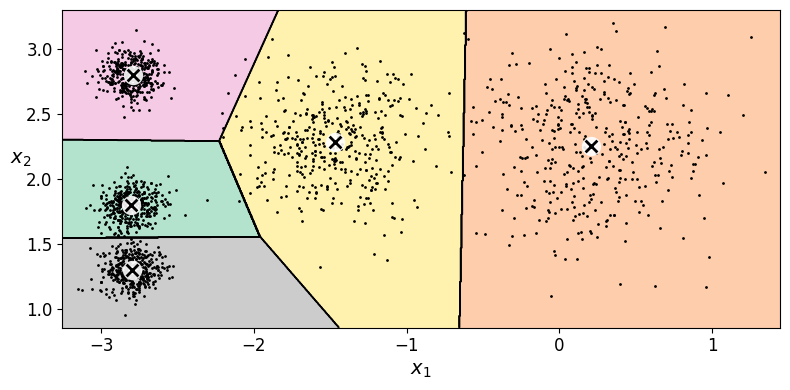
17.1.1. Decision Boundaries#
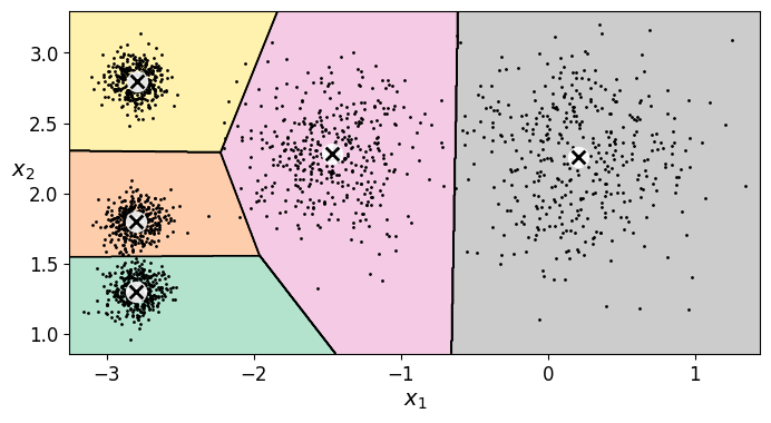
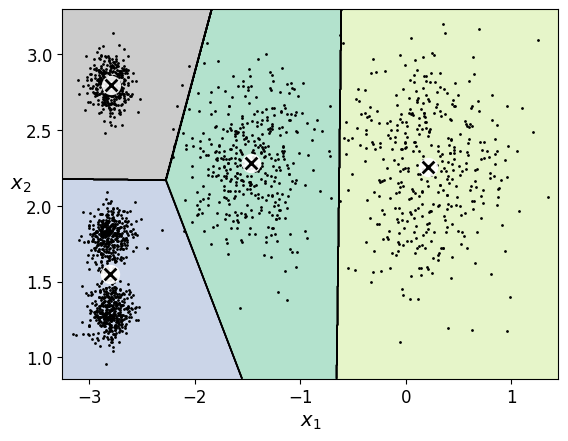
Let’s plot the model’s decision boundaries. This gives us a Voronoi diagram:
def plot_data(X):
    plt.plot(X[:, 0], X[:, 1], 'k.', markersize=2)

def plot_centroids(centroids, weights=None, circle_color='w', cross_color='k'):
    if weights is not None:
        centroids = centroids[weights > weights.max() / 10]
    plt.scatter(centroids[:, 0], centroids[:, 1],
                marker='o', s=35, linewidths=8,
                color=circle_color, zorder=10, alpha=0.9)
    plt.scatter(centroids[:, 0], centroids[:, 1],
                marker='x', s=2, linewidths=12,
                color=cross_color, zorder=11, alpha=1)

def plot_decision_boundaries(clusterer, X, resolution=1000, show_centroids=True,
                             show_xlabels=True, show_ylabels=True):
    mins = X.min(axis=0) - 0.1
    maxs = X.max(axis=0) + 0.1
    xx, yy = np.meshgrid(np.linspace(mins[0], maxs[0], resolution),
                         np.linspace(mins[1], maxs[1], resolution))
    Z = clusterer.predict(np.c_[xx.ravel(), yy.ravel()])
    Z = Z.reshape(xx.shape)

    plt.contourf(Z, extent=(mins[0], maxs[0], mins[1], maxs[1]),
                cmap="Pastel2")
    plt.contour(Z, extent=(mins[0], maxs[0], mins[1], maxs[1]),
                linewidths=1, colors='k')
    plot_data(X)
    if show_centroids:
        plot_centroids(clusterer.cluster_centers_)

    if show_xlabels:
        plt.xlabel("$x_1$", fontsize=14)
    else:
        plt.tick_params(labelbottom=False)
    if show_ylabels:
        plt.ylabel("$x_2$", fontsize=14, rotation=0)
    else:
        plt.tick_params(labelleft=False)
plt.figure(figsize=(8, 4))
plot_decision_boundaries(kmeans, X)
save_fig("voronoi_plot")
plt.show()
Saving figure voronoi_plot
Hard Clustering vs Soft Clustering
kmeans.transform(X_new)
array([[2.81093633, 0.32995317, 2.9042344 , 1.49439034, 2.88633901],
       [5.80730058, 2.80290755, 5.84739223, 4.4759332 , 5.84236351],
       [1.21475352, 3.29399768, 0.29040966, 1.69136631, 1.71086031],
       [0.72581411, 3.21806371, 0.36159148, 1.54808703, 1.21567622]])
You can verify that this is indeed the Euclidian distance between each instance and each centroid:
np.linalg.norm(np.tile(X_new, (1, k)).reshape(-1, k, 2) - kmeans.cluster_centers_, axis=2)
array([[2.81093633, 0.32995317, 2.9042344 , 1.49439034, 2.88633901],
       [5.80730058, 2.80290755, 5.84739223, 4.4759332 , 5.84236351],
       [1.21475352, 3.29399768, 0.29040966, 1.69136631, 1.71086031],
       [0.72581411, 3.21806371, 0.36159148, 1.54808703, 1.21567622]])
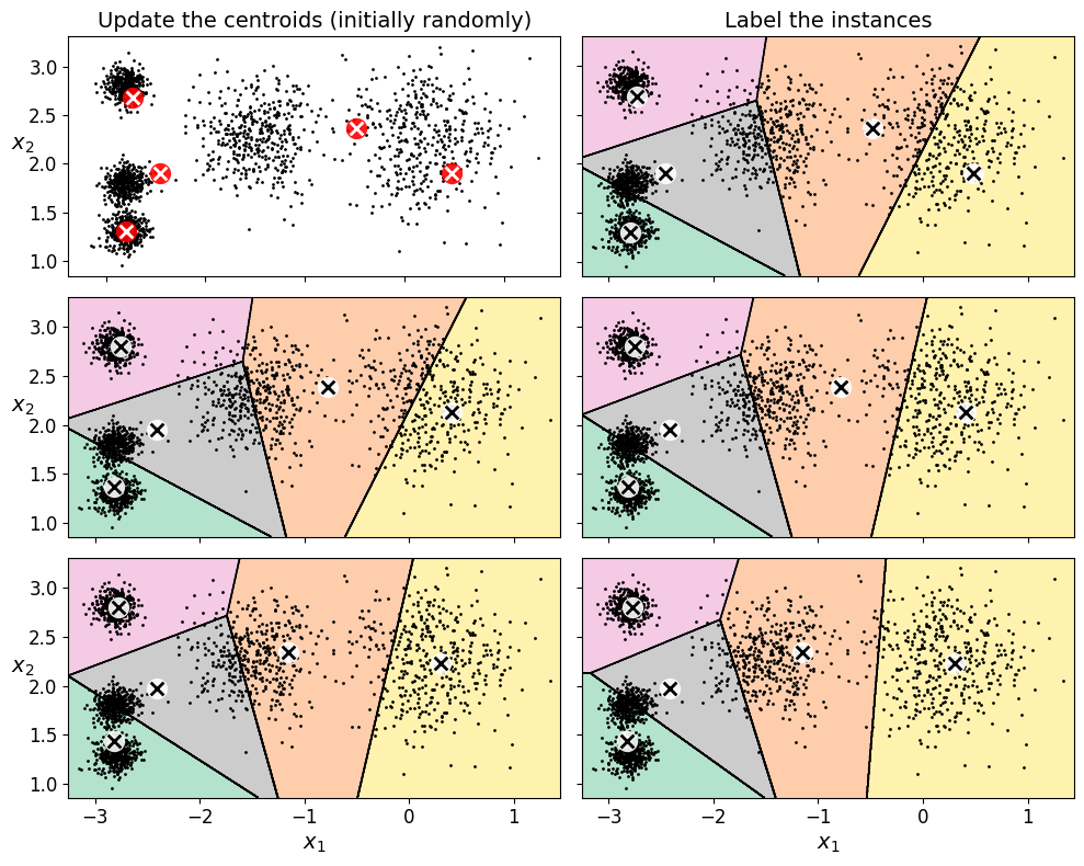
17.1.2. The K-Means Algorithm#
The KMeans class applies an optimized algorithm by default. To get the original K-Means algorithm (for educational purposes only), you must set init=“random”, n_init=1 and algorithm=“full”. These hyperparameters will be explained below.
Let’s run the K-Means algorithm for 1, 2 and 3 iterations, to see how the centroids move around:
kmeans_iter1 = KMeans(n_clusters=5, init="random", n_init=1,
                     algorithm="full", max_iter=1, random_state=0)
kmeans_iter2 = KMeans(n_clusters=5, init="random", n_init=1,
                     algorithm="full", max_iter=2, random_state=0)
kmeans_iter3 = KMeans(n_clusters=5, init="random", n_init=1,
                     algorithm="full", max_iter=3, random_state=0)
kmeans_iter1.fit(X)
kmeans_iter2.fit(X)
kmeans_iter3.fit(X)
KMeans(algorithm='full', init='random', max_iter=3, n_clusters=5, n_init=1,
       random_state=0)
In a Jupyter environment, please rerun this cell to show the HTML representation or trust the notebook. On GitHub, the HTML representation is unable to render, please try loading this page with nbviewer.org.
KMeans(algorithm='full', init='random', max_iter=3, n_clusters=5, n_init=1,
       random_state=0)
And let’s plot this:
plt.figure(figsize=(10, 8))

plt.subplot(321)
plot_data(X)
plot_centroids(kmeans_iter1.cluster_centers_, circle_color='r', cross_color='w')
plt.ylabel("$x_2$", fontsize=14, rotation=0)
plt.tick_params(labelbottom=False)
plt.title("Update the centroids (initially randomly)", fontsize=14)

plt.subplot(322)
plot_decision_boundaries(kmeans_iter1, X, show_xlabels=False, show_ylabels=False)
plt.title("Label the instances", fontsize=14)

plt.subplot(323)
plot_decision_boundaries(kmeans_iter1, X, show_centroids=False, show_xlabels=False)
plot_centroids(kmeans_iter2.cluster_centers_)

plt.subplot(324)
plot_decision_boundaries(kmeans_iter2, X, show_xlabels=False, show_ylabels=False)

plt.subplot(325)
plot_decision_boundaries(kmeans_iter2, X, show_centroids=False)
plot_centroids(kmeans_iter3.cluster_centers_)

plt.subplot(326)
plot_decision_boundaries(kmeans_iter3, X, show_ylabels=False)

save_fig("kmeans_algorithm_plot")
plt.show()
Saving figure kmeans_algorithm_plot
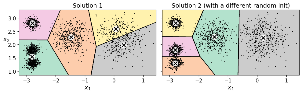
17.1.3. K-Means Variability#
In the original K-Means algorithm, the centroids are just initialized randomly, and the algorithm simply runs a single iteration to gradually improve the centroids, as we saw above.
However, one major problem with this approach is that if you run K-Means multiple times (or with different random seeds), it can converge to very different solutions, as you can see below:
def plot_clusterer_comparison(clusterer1, clusterer2, X, title1=None, title2=None):
    clusterer1.fit(X)
    clusterer2.fit(X)

    plt.figure(figsize=(10, 3.2))

    plt.subplot(121)
    plot_decision_boundaries(clusterer1, X)
    if title1:
        plt.title(title1, fontsize=14)

    plt.subplot(122)
    plot_decision_boundaries(clusterer2, X, show_ylabels=False)
    if title2:
        plt.title(title2, fontsize=14)
kmeans_rnd_init1 = KMeans(n_clusters=5, init="random", n_init=1,
                         algorithm="full", random_state=2)
kmeans_rnd_init2 = KMeans(n_clusters=5, init="random", n_init=1,
                         algorithm="full", random_state=5)

plot_clusterer_comparison(kmeans_rnd_init1, kmeans_rnd_init2, X,
                          "Solution 1", "Solution 2 (with a different random init)")

save_fig("kmeans_variability_plot")
plt.show()
Saving figure kmeans_variability_plot
17.1.4. Inertia#
To select the best model, we will need a way to evaluate a K-Mean model’s performance. Unfortunately, clustering is an unsupervised task, so we do not have the targets. But at least we can measure the distance between each instance and its centroid. This is the idea behind the inertia metric:
kmeans.inertia_
211.5985372581684
As you can easily verify, inertia is the sum of the squared distances between each training instance and its closest centroid:
X_dist = kmeans.transform(X)
np.sum(X_dist[np.arange(len(X_dist)), kmeans.labels_]**2)
211.59853725816868
The score() method returns the negative inertia. Why negative? Well, it is because a predictor’s score() method must always respect the “greater is better” rule.
kmeans.score(X)
-211.59853725816836
17.1.5. Multiple Initializations#
So one approach to solve the variability issue is to simply run the K-Means algorithm multiple times with different random initializations, and select the solution that minimizes the inertia. For example, here are the inertias of the two “bad” models shown in the previous figure:
kmeans_rnd_init1.inertia_
219.43539442771396
kmeans_rnd_init2.inertia_
211.5985372581684
As you can see, they have a higher inertia than the first “good” model we trained, which means they are probably worse.
When you set the n_init hyperparameter, Scikit-Learn runs the original algorithm n_init times, and selects the solution that minimizes the inertia. By default, Scikit-Learn sets n_init=10.
kmeans_rnd_10_inits = KMeans(n_clusters=5, init="random", n_init=10,
                              algorithm="full", random_state=2)
kmeans_rnd_10_inits.fit(X)
KMeans(algorithm='full', init='random', n_clusters=5, n_init=10, random_state=2)In a Jupyter environment, please rerun this cell to show the HTML representation or trust the notebook.
On GitHub, the HTML representation is unable to render, please try loading this page with nbviewer.org.
KMeans(algorithm='full', init='random', n_clusters=5, n_init=10, random_state=2)
As you can see, we end up with the initial model, which is certainly the optimal K-Means solution (at least in terms of inertia, and assuming \(k=5\)).
plt.figure(figsize=(8, 4))
plot_decision_boundaries(kmeans_rnd_10_inits, X)
plt.show()
17.1.6. Centroid initialization methods#
Instead of initializing the centroids entirely randomly, it is preferable to initialize them using the following algorithm, proposed in a 2006 paper by David Arthur and Sergei Vassilvitskii:
Take one centroid \(c_1\), chosen uniformly at random from the dataset.
Take a new center \(c_i\), choosing an instance \(\mathbf{x}_i\) with probability: \(D(\mathbf{x}_i)^2\) / \(\sum\limits_{j=1}^{m}{D(\mathbf{x}_j)}^2\) where \(D(\mathbf{x}_i)\) is the distance between the instance \(\mathbf{x}_i\) and the closest centroid that was already chosen. This probability distribution ensures that instances that are further away from already chosen centroids are much more likely be selected as centroids.
Repeat the previous step until all \(k\) centroids have been chosen.
The rest of the K-Means++ algorithm is just regular K-Means. With this initialization, the K-Means algorithm is much less likely to converge to a suboptimal solution, so it is possible to reduce n_init considerably. Most of the time, this largely compensates for the additional complexity of the initialization process.
To set the initialization to K-Means++, simply set init="k-means++" (this is actually the default):
KMeans()
KMeans()In a Jupyter environment, please rerun this cell to show the HTML representation or trust the notebook.
On GitHub, the HTML representation is unable to render, please try loading this page with nbviewer.org.
KMeans()
good_init = np.array([[-3, 3], [-3, 2], [-3, 1], [-1, 2], [0, 2]])
kmeans = KMeans(n_clusters=5, init=good_init, n_init=1, random_state=42)
kmeans.fit(X)
kmeans.inertia_
211.5985372581684
17.1.7. Accelerated K-Means#
The K-Means algorithm can be significantly accelerated by avoiding many unnecessary distance calculations: this is achieved by exploiting the triangle inequality (given three points A, B and C, the distance AC is always such that AC ≤ AB + BC) and by keeping track of lower and upper bounds for distances between instances and centroids.
%timeit -n 50 KMeans(algorithm="elkan", random_state=42).fit(X)
The slowest run took 7.79 times longer than the fastest. This could mean that an intermediate result is being cached.
135 ms ± 134 ms per loop (mean ± std. dev. of 7 runs, 50 loops each)
%timeit -n 50 KMeans(algorithm="full", random_state=42).fit(X)
43 ms ± 14.6 ms per loop (mean ± std. dev. of 7 runs, 50 loops each)
There’s no big difference in this case, as the dataset is fairly small.
17.1.8. Mini-Batch K-Means#
Scikit-Learn also implements a variant of the K-Means algorithm that supports mini-batches.
from sklearn.cluster import MiniBatchKMeans
minibatch_kmeans = MiniBatchKMeans(n_clusters=5, random_state=42)
minibatch_kmeans.fit(X)
MiniBatchKMeans(n_clusters=5, random_state=42)In a Jupyter environment, please rerun this cell to show the HTML representation or trust the notebook.
On GitHub, the HTML representation is unable to render, please try loading this page with nbviewer.org.
MiniBatchKMeans(n_clusters=5, random_state=42)
minibatch_kmeans.inertia_
211.65239850433215
17.2. PCA#
If the dataset does not fit in memory, the simplest option is to use the memmap class, just like we did for incremental PCA in the previous chapter. First let’s load MNIST:
Warning: since Scikit-Learn 0.24, fetch_openml() returns a Pandas DataFrame by default. To avoid this and keep the same code as in the book, we use as_frame=False.
import urllib.request
from sklearn.datasets import fetch_openml

mnist = fetch_openml('mnist_784', version=1, as_frame=False)
mnist.target = mnist.target.astype(np.int64)
from sklearn.model_selection import train_test_split

X_train, X_test, y_train, y_test = train_test_split(
    mnist["data"], mnist["target"], random_state=42)
filename = "my_mnist.data"
X_mm = np.memmap(filename, dtype='float32', mode='write', shape=X_train.shape)
X_mm[:] = X_train
minibatch_kmeans = MiniBatchKMeans(n_clusters=10, batch_size=10, random_state=42)
minibatch_kmeans.fit(X_mm)
MiniBatchKMeans(batch_size=10, n_clusters=10, random_state=42)In a Jupyter environment, please rerun this cell to show the HTML representation or trust the notebook.
On GitHub, the HTML representation is unable to render, please try loading this page with nbviewer.org.
MiniBatchKMeans(batch_size=10, n_clusters=10, random_state=42)
If your data is so large that you cannot use memmap, things get more complicated. Let’s start by writing a function to load the next batch (in real life, you would load the data from disk):
def load_next_batch(batch_size):
    return X[np.random.choice(len(X), batch_size, replace=False)]
Now we can train the model by feeding it one batch at a time. We also need to implement multiple initializations and keep the model with the lowest inertia:
np.random.seed(42)
k = 5
n_init = 10
n_iterations = 100
batch_size = 100
init_size = 500  # more data for K-Means++ initialization
evaluate_on_last_n_iters = 10

best_kmeans = None

for init in range(n_init):
    minibatch_kmeans = MiniBatchKMeans(n_clusters=k, init_size=init_size)
    X_init = load_next_batch(init_size)
    minibatch_kmeans.partial_fit(X_init)

    minibatch_kmeans.sum_inertia_ = 0
    for iteration in range(n_iterations):
        X_batch = load_next_batch(batch_size)
        minibatch_kmeans.partial_fit(X_batch)
        if iteration >= n_iterations - evaluate_on_last_n_iters:
            minibatch_kmeans.sum_inertia_ += minibatch_kmeans.inertia_

    if (best_kmeans is None or
        minibatch_kmeans.sum_inertia_ < best_kmeans.sum_inertia_):
        best_kmeans = minibatch_kmeans
best_kmeans.score(X)
-211.62571878891146
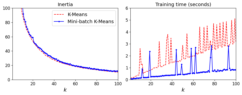
Mini-batch K-Means is much faster than regular K-Means:
%timeit KMeans(n_clusters=5, random_state=42).fit(X)
23.9 ms ± 1.4 ms per loop (mean ± std. dev. of 7 runs, 10 loops each)
%timeit MiniBatchKMeans(n_clusters=5, random_state=42).fit(X)
13.5 ms ± 7.84 ms per loop (mean ± std. dev. of 7 runs, 100 loops each)
That’s much faster! However, its performance is often lower (higher inertia), and it keeps degrading as k increases. Let’s plot the inertia ratio and the training time ratio between Mini-batch K-Means and regular K-Means:
from timeit import timeit
times = np.empty((100, 2))
inertias = np.empty((100, 2))
for k in range(1, 101):
    kmeans_ = KMeans(n_clusters=k, random_state=42)
    minibatch_kmeans = MiniBatchKMeans(n_clusters=k, random_state=42)
    print("\r{}/{}".format(k, 100), end="")
    times[k-1, 0] = timeit("kmeans_.fit(X)", number=10, globals=globals())
    times[k-1, 1]  = timeit("minibatch_kmeans.fit(X)", number=10, globals=globals())
    inertias[k-1, 0] = kmeans_.inertia_
    inertias[k-1, 1] = minibatch_kmeans.inertia_
100/100
plt.figure(figsize=(10,4))

plt.subplot(121)
plt.plot(range(1, 101), inertias[:, 0], "r--", label="K-Means")
plt.plot(range(1, 101), inertias[:, 1], "b.-", label="Mini-batch K-Means")
plt.xlabel("$k$", fontsize=16)
plt.title("Inertia", fontsize=14)
plt.legend(fontsize=14)
plt.axis([1, 100, 0, 100])

plt.subplot(122)
plt.plot(range(1, 101), times[:, 0], "r--", label="K-Means")
plt.plot(range(1, 101), times[:, 1], "b.-", label="Mini-batch K-Means")
plt.xlabel("$k$", fontsize=16)
plt.title("Training time (seconds)", fontsize=14)
plt.axis([1, 100, 0, 6])

save_fig("minibatch_kmeans_vs_kmeans")
plt.show()
Saving figure minibatch_kmeans_vs_kmeans
17.2.1. Finding the optimal number of clusters#
What if the number of clusters was set to a lower or greater value than 5?
kmeans_k3 = KMeans(n_clusters=3, random_state=42)
kmeans_k8 = KMeans(n_clusters=8, random_state=42)

plot_clusterer_comparison(kmeans_k3, kmeans_k8, X, "$k=3$", "$k=8$")
save_fig("bad_n_clusters_plot")
plt.show()
Saving figure bad_n_clusters_plot
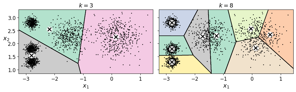
Ouch, these two models don’t look great. What about their inertias?
kmeans_k3.inertia_
653.216719002155
kmeans_k8.inertia_
119.11983416102879
No, we cannot simply take the value of \(k\) that minimizes the inertia, since it keeps getting lower as we increase \(k\). Indeed, the more clusters there are, the closer each instance will be to its closest centroid, and therefore the lower the inertia will be. However, we can plot the inertia as a function of \(k\) and analyze the resulting curve:
kmeans_per_k = [KMeans(n_clusters=k, random_state=42).fit(X)
                for k in range(1, 10)]
inertias = [model.inertia_ for model in kmeans_per_k]
plt.figure(figsize=(8, 3.5))
plt.plot(range(1, 10), inertias, "bo-")
plt.xlabel("$k$", fontsize=14)
plt.ylabel("Inertia", fontsize=14)
plt.annotate('Elbow',
             xy=(4, inertias[3]),
             xytext=(0.55, 0.55),
             textcoords='figure fraction',
             fontsize=16,
             arrowprops=dict(facecolor='black', shrink=0.1)
            )
plt.axis([1, 8.5, 0, 1300])
save_fig("inertia_vs_k_plot")
plt.show()
Saving figure inertia_vs_k_plot
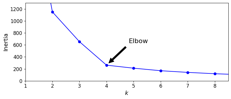
As you can see, there is an elbow at \(k=4\), which means that less clusters than that would be bad, and more clusters would not help much and might cut clusters in half. So \(k=4\) is a pretty good choice. Of course in this example it is not perfect since it means that the two blobs in the lower left will be considered as just a single cluster, but it’s a pretty good clustering nonetheless.
plot_decision_boundaries(kmeans_per_k[4-1], X)
plt.show()
Another approach is to look at the silhouette score, which is the mean silhouette coefficient over all the instances. An instance’s silhouette coefficient is equal to \((b - a)/\max(a, b)\) where \(a\) is the mean distance to the other instances in the same cluster (it is the mean intra-cluster distance), and \(b\) is the mean nearest-cluster distance, that is the mean distance to the instances of the next closest cluster (defined as the one that minimizes \(b\), excluding the instance’s own cluster). The silhouette coefficient can vary between -1 and +1: a coefficient close to +1 means that the instance is well inside its own cluster and far from other clusters, while a coefficient close to 0 means that it is close to a cluster boundary, and finally a coefficient close to -1 means that the instance may have been assigned to the wrong cluster.
Let’s plot the silhouette score as a function of \(k\):
from sklearn.metrics import silhouette_score
silhouette_score(X, kmeans.labels_)
0.655517642572828
silhouette_scores = [silhouette_score(X, model.labels_)
                     for model in kmeans_per_k[1:]]
plt.figure(figsize=(8, 3))
plt.plot(range(2, 10), silhouette_scores, "bo-")
plt.xlabel("$k$", fontsize=14)
plt.ylabel("Silhouette score", fontsize=14)
plt.axis([1.8, 8.5, 0.55, 0.7])
save_fig("silhouette_score_vs_k_plot")
plt.show()
Saving figure silhouette_score_vs_k_plot
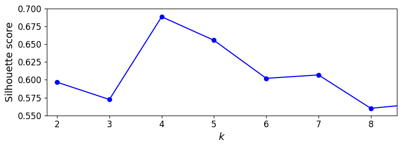
As you can see, this visualization is much richer than the previous one: in particular, although it confirms that \(k=4\) is a very good choice, but it also underlines the fact that \(k=5\) is quite good as well.
An even more informative visualization is given when you plot every instance’s silhouette coefficient, sorted by the cluster they are assigned to and by the value of the coefficient. This is called a silhouette diagram:
from sklearn.metrics import silhouette_samples
from matplotlib.ticker import FixedLocator, FixedFormatter

plt.figure(figsize=(11, 9))

for k in (3, 4, 5, 6):
    plt.subplot(2, 2, k - 2)

    y_pred = kmeans_per_k[k - 1].labels_
    silhouette_coefficients = silhouette_samples(X, y_pred)

    padding = len(X) // 30
    pos = padding
    ticks = []
    for i in range(k):
        coeffs = silhouette_coefficients[y_pred == i]
        coeffs.sort()

        color = mpl.cm.Spectral(i / k)
        plt.fill_betweenx(np.arange(pos, pos + len(coeffs)), 0, coeffs,
                          facecolor=color, edgecolor=color, alpha=0.7)
        ticks.append(pos + len(coeffs) // 2)
        pos += len(coeffs) + padding

    plt.gca().yaxis.set_major_locator(FixedLocator(ticks))
    plt.gca().yaxis.set_major_formatter(FixedFormatter(range(k)))
    if k in (3, 5):
        plt.ylabel("Cluster")

    if k in (5, 6):
        plt.gca().set_xticks([-0.1, 0, 0.2, 0.4, 0.6, 0.8, 1])
        plt.xlabel("Silhouette Coefficient")
    else:
        plt.tick_params(labelbottom=False)

    plt.axvline(x=silhouette_scores[k - 2], color="red", linestyle="--")
    plt.title("$k={}$".format(k), fontsize=16)

save_fig("silhouette_analysis_plot")
plt.show()
Saving figure silhouette_analysis_plot
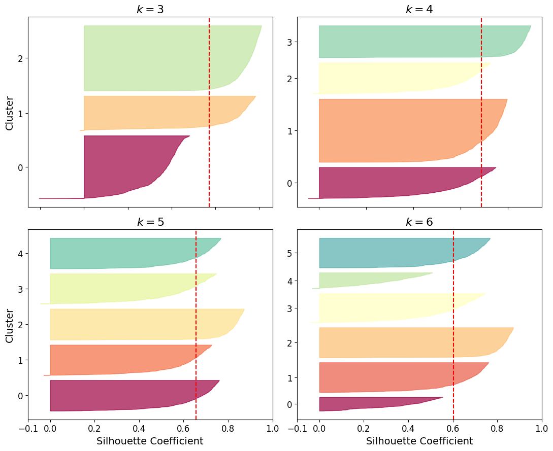
As you can see, \(k=5\) looks like the best option here, as all clusters are roughly the same size, and they all cross the dashed line, which represents the mean silhouette score.
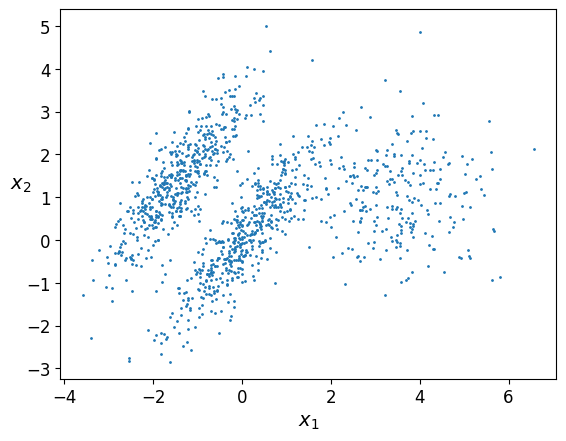
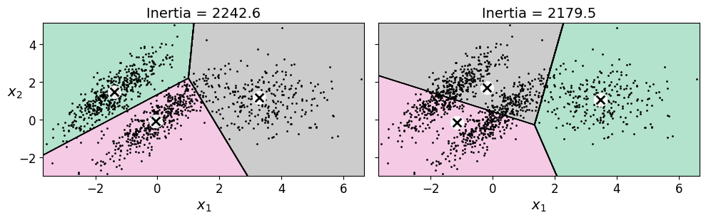
17.2.2. Limits of K-Means#
X1, y1 = make_blobs(n_samples=1000, centers=((4, -4), (0, 0)), random_state=42)
X1 = X1.dot(np.array([[0.374, 0.95], [0.732, 0.598]]))
X2, y2 = make_blobs(n_samples=250, centers=1, random_state=42)
X2 = X2 + [6, -8]
X = np.r_[X1, X2]
y = np.r_[y1, y2]
plot_clusters(X)
kmeans_good = KMeans(n_clusters=3, init=np.array([[-1.5, 2.5], [0.5, 0], [4, 0]]), n_init=1, random_state=42)
kmeans_bad = KMeans(n_clusters=3, random_state=42)
kmeans_good.fit(X)
kmeans_bad.fit(X)
KMeans(n_clusters=3, random_state=42)In a Jupyter environment, please rerun this cell to show the HTML representation or trust the notebook.
On GitHub, the HTML representation is unable to render, please try loading this page with nbviewer.org.
KMeans(n_clusters=3, random_state=42)
plt.figure(figsize=(10, 3.2))

plt.subplot(121)
plot_decision_boundaries(kmeans_good, X)
plt.title("Inertia = {:.1f}".format(kmeans_good.inertia_), fontsize=14)

plt.subplot(122)
plot_decision_boundaries(kmeans_bad, X, show_ylabels=False)
plt.title("Inertia = {:.1f}".format(kmeans_bad.inertia_), fontsize=14)

save_fig("bad_kmeans_plot")
plt.show()
Saving figure bad_kmeans_plot
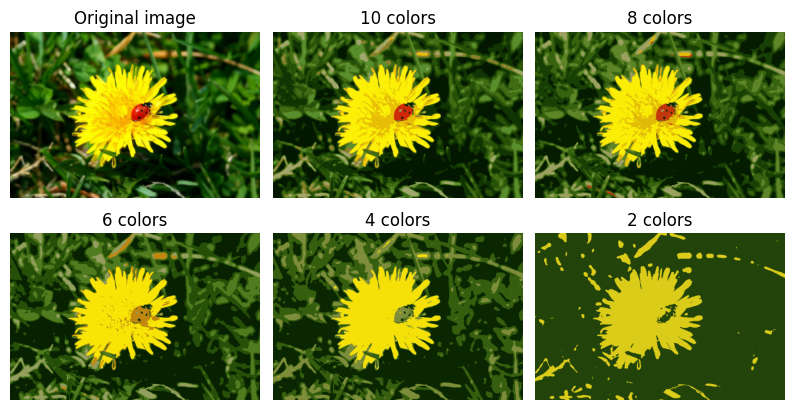
17.2.3. Using Clustering for Image Segmentation#
# Download the ladybug image
images_path = os.path.join(PROJECT_ROOT_DIR, "images", "unsupervised_learning")
os.makedirs(images_path, exist_ok=True)
DOWNLOAD_ROOT = "https://raw.githubusercontent.com/ageron/handson-ml2/master/"
filename = "ladybug.png"
print("Downloading", filename)
url = DOWNLOAD_ROOT + "images/unsupervised_learning/" + filename
urllib.request.urlretrieve(url, os.path.join(images_path, filename))
Downloading ladybug.png
('./images/unsupervised_learning/ladybug.png',
 <http.client.HTTPMessage at 0x7e1538110d60>)
from matplotlib.image import imread
image = imread(os.path.join(images_path, filename))
image.shape
(533, 800, 3)
X = image.reshape(-1, 3)
kmeans = KMeans(n_clusters=8, random_state=42).fit(X)
segmented_img = kmeans.cluster_centers_[kmeans.labels_]
segmented_img = segmented_img.reshape(image.shape)
segmented_imgs = []
n_colors = (10, 8, 6, 4, 2)
for n_clusters in n_colors:
    kmeans = KMeans(n_clusters=n_clusters, random_state=42).fit(X)
    segmented_img = kmeans.cluster_centers_[kmeans.labels_]
    segmented_imgs.append(segmented_img.reshape(image.shape))
plt.figure(figsize=(10,5))
plt.subplots_adjust(wspace=0.05, hspace=0.1)

plt.subplot(231)
plt.imshow(image)
plt.title("Original image")
plt.axis('off')

for idx, n_clusters in enumerate(n_colors):
    plt.subplot(232 + idx)
    plt.imshow(segmented_imgs[idx])
    plt.title("{} colors".format(n_clusters))
    plt.axis('off')

save_fig('image_segmentation_diagram', tight_layout=False)
plt.show()
Saving figure image_segmentation_diagram
17.2.4. Using Clustering for Preprocessing#
Let’s tackle the digits dataset which is a simple MNIST-like dataset containing 1,797 grayscale 8×8 images representing digits 0 to 9.
from sklearn.datasets import load_digits
X_digits, y_digits = load_digits(return_X_y=True)
Let’s split it into a training set and a test set:
from sklearn.model_selection import train_test_split
X_train, X_test, y_train, y_test = train_test_split(X_digits, y_digits, random_state=42)
17.3. LDA#
from IPython.display import HTML
display(HTML("""
<p style="text-align: center;">
<iframe src="https://static-1300131294.cos.ap-shanghai.myqcloud.com/html/t-SNE-demo/t-SNE.html" width="105%" height="800px;"
style="border:none;" scrolling="auto"></iframe>
A demo of linear-regression. <a
href="http://alekseynp.com/viz/k-means.html"> [source]</a>
</p>
"""))
A demo of linear-regression. [source]
from sklearn.linear_model import LogisticRegression
log_reg = LogisticRegression(multi_class="ovr", solver="lbfgs", max_iter=5000, random_state=42)
log_reg.fit(X_train, y_train)
LogisticRegression(max_iter=5000, multi_class='ovr', random_state=42)In a Jupyter environment, please rerun this cell to show the HTML representation or trust the notebook.
On GitHub, the HTML representation is unable to render, please try loading this page with nbviewer.org.
LogisticRegression(max_iter=5000, multi_class='ovr', random_state=42)
log_reg_score = log_reg.score(X_test, y_test)
log_reg_score
0.9688888888888889
Okay, that’s our baseline: 96.89% accuracy. Let’s see if we can do better by using K-Means as a preprocessing step. We will create a pipeline that will first cluster the training set into 50 clusters and replace the images with their distances to the 50 clusters, then apply a logistic regression model:
from sklearn.pipeline import Pipeline
pipeline = Pipeline([
    ("kmeans", KMeans(n_clusters=50, random_state=42)),
    ("log_reg", LogisticRegression(multi_class="ovr", solver="lbfgs", max_iter=5000, random_state=42)),
])
pipeline.fit(X_train, y_train)
Pipeline(steps=[('kmeans', KMeans(n_clusters=50, random_state=42)),
                ('log_reg',
                 LogisticRegression(max_iter=5000, multi_class='ovr',
                                    random_state=42))])
In a Jupyter environment, please rerun this cell to show the HTML representation or trust the notebook. On GitHub, the HTML representation is unable to render, please try loading this page with nbviewer.org.
Pipeline(steps=[('kmeans', KMeans(n_clusters=50, random_state=42)),
                ('log_reg',
                 LogisticRegression(max_iter=5000, multi_class='ovr',
random_state=42))])KMeans(n_clusters=50, random_state=42)
LogisticRegression(max_iter=5000, multi_class='ovr', random_state=42)
pipeline_score = pipeline.score(X_test, y_test)
pipeline_score
0.9777777777777777
How much did the error rate drop?
1 - (1 - pipeline_score) / (1 - log_reg_score)
0.28571428571428414
How about that? We reduced the error rate by over 35%! But we chose the number of clusters \(k\) completely arbitrarily, we can surely do better. Since K-Means is just a preprocessing step in a classification pipeline, finding a good value for \(k\) is much simpler than earlier: there’s no need to perform silhouette analysis or minimize the inertia, the best value of \(k\) is simply the one that results in the best classification performance.
from sklearn.model_selection import GridSearchCV
Warning: the following cell may take close to 20 minutes to run, or more depending on your hardware.
param_grid = dict(kmeans__n_clusters=range(2, 100))
grid_clf = GridSearchCV(pipeline, param_grid, cv=3, verbose=2)
grid_clf.fit(X_train, y_train)
Fitting 3 folds for each of 98 candidates, totalling 294 fits
[CV] END ...............................kmeans__n_clusters=2; total time=   0.6s
[CV] END ...............................kmeans__n_clusters=2; total time=   1.2s
[CV] END ...............................kmeans__n_clusters=2; total time=   1.7s
[CV] END ...............................kmeans__n_clusters=3; total time=   0.6s
[CV] END ...............................kmeans__n_clusters=3; total time=   0.8s
[CV] END ...............................kmeans__n_clusters=3; total time=   0.7s
[CV] END ...............................kmeans__n_clusters=4; total time=   0.7s
[CV] END ...............................kmeans__n_clusters=4; total time=   0.5s
[CV] END ...............................kmeans__n_clusters=4; total time=   0.7s
[CV] END ...............................kmeans__n_clusters=5; total time=   0.7s
[CV] END ...............................kmeans__n_clusters=5; total time=   0.7s
[CV] END ...............................kmeans__n_clusters=5; total time=   0.5s
[CV] END ...............................kmeans__n_clusters=6; total time=   0.7s
[CV] END ...............................kmeans__n_clusters=6; total time=   0.9s
[CV] END ...............................kmeans__n_clusters=6; total time=   0.6s
[CV] END ...............................kmeans__n_clusters=7; total time=   0.7s
[CV] END ...............................kmeans__n_clusters=7; total time=   0.8s
[CV] END ...............................kmeans__n_clusters=7; total time=   2.4s
[CV] END ...............................kmeans__n_clusters=8; total time=   0.8s
[CV] END ...............................kmeans__n_clusters=8; total time=   0.8s
[CV] END ...............................kmeans__n_clusters=8; total time=   0.9s
[CV] END ...............................kmeans__n_clusters=9; total time=   0.8s
[CV] END ...............................kmeans__n_clusters=9; total time=   1.1s
[CV] END ...............................kmeans__n_clusters=9; total time=   1.1s
[CV] END ..............................kmeans__n_clusters=10; total time=   1.0s
[CV] END ..............................kmeans__n_clusters=10; total time=   1.1s
[CV] END ..............................kmeans__n_clusters=10; total time=   1.3s
[CV] END ..............................kmeans__n_clusters=11; total time=   1.7s
[CV] END ..............................kmeans__n_clusters=11; total time=   2.4s
[CV] END ..............................kmeans__n_clusters=11; total time=   1.9s
[CV] END ..............................kmeans__n_clusters=12; total time=   1.6s
[CV] END ..............................kmeans__n_clusters=12; total time=   1.5s
[CV] END ..............................kmeans__n_clusters=12; total time=   1.6s
[CV] END ..............................kmeans__n_clusters=13; total time=   1.5s
[CV] END ..............................kmeans__n_clusters=13; total time=   1.6s
[CV] END ..............................kmeans__n_clusters=13; total time=   2.6s
[CV] END ..............................kmeans__n_clusters=14; total time=   2.9s
[CV] END ..............................kmeans__n_clusters=14; total time=   1.7s
[CV] END ..............................kmeans__n_clusters=14; total time=   1.8s
[CV] END ..............................kmeans__n_clusters=15; total time=   2.2s
[CV] END ..............................kmeans__n_clusters=15; total time=   2.0s
[CV] END ..............................kmeans__n_clusters=15; total time=   3.9s
[CV] END ..............................kmeans__n_clusters=16; total time=   2.2s
[CV] END ..............................kmeans__n_clusters=16; total time=   2.2s
[CV] END ..............................kmeans__n_clusters=16; total time=   2.3s
[CV] END ..............................kmeans__n_clusters=17; total time=   2.4s
[CV] END ..............................kmeans__n_clusters=17; total time=   4.2s
[CV] END ..............................kmeans__n_clusters=17; total time=   2.4s
[CV] END ..............................kmeans__n_clusters=18; total time=   2.6s
[CV] END ..............................kmeans__n_clusters=18; total time=   2.6s
[CV] END ..............................kmeans__n_clusters=18; total time=   2.5s
[CV] END ..............................kmeans__n_clusters=19; total time=   4.1s
[CV] END ..............................kmeans__n_clusters=19; total time=   2.7s
[CV] END ..............................kmeans__n_clusters=19; total time=   2.6s
[CV] END ..............................kmeans__n_clusters=20; total time=   2.8s
[CV] END ..............................kmeans__n_clusters=20; total time=   6.5s
[CV] END ..............................kmeans__n_clusters=20; total time=   2.5s
[CV] END ..............................kmeans__n_clusters=21; total time=   2.9s
[CV] END ..............................kmeans__n_clusters=21; total time=   2.9s
[CV] END ..............................kmeans__n_clusters=21; total time=   3.4s
[CV] END ..............................kmeans__n_clusters=22; total time=   3.6s
[CV] END ..............................kmeans__n_clusters=22; total time=   3.1s
[CV] END ..............................kmeans__n_clusters=22; total time=   2.8s
[CV] END ..............................kmeans__n_clusters=23; total time=   3.7s
[CV] END ..............................kmeans__n_clusters=23; total time=   3.8s
[CV] END ..............................kmeans__n_clusters=23; total time=   2.7s
[CV] END ..............................kmeans__n_clusters=24; total time=   3.0s
[CV] END ..............................kmeans__n_clusters=24; total time=   5.3s
[CV] END ..............................kmeans__n_clusters=24; total time=   2.7s
[CV] END ..............................kmeans__n_clusters=25; total time=   2.6s
[CV] END ..............................kmeans__n_clusters=25; total time=   2.8s
[CV] END ..............................kmeans__n_clusters=25; total time=   3.9s
[CV] END ..............................kmeans__n_clusters=26; total time=   3.6s
[CV] END ..............................kmeans__n_clusters=26; total time=   3.5s
[CV] END ..............................kmeans__n_clusters=26; total time=   2.5s
[CV] END ..............................kmeans__n_clusters=27; total time=   4.2s
[CV] END ..............................kmeans__n_clusters=27; total time=   3.5s
[CV] END ..............................kmeans__n_clusters=27; total time=   2.9s
[CV] END ..............................kmeans__n_clusters=28; total time=   3.8s
[CV] END ..............................kmeans__n_clusters=28; total time=   5.1s
[CV] END ..............................kmeans__n_clusters=28; total time=   2.9s
[CV] END ..............................kmeans__n_clusters=29; total time=   2.7s
[CV] END ..............................kmeans__n_clusters=29; total time=   3.9s
[CV] END ..............................kmeans__n_clusters=29; total time=   4.7s
[CV] END ..............................kmeans__n_clusters=30; total time=   3.3s
[CV] END ..............................kmeans__n_clusters=30; total time=   3.1s
[CV] END ..............................kmeans__n_clusters=30; total time=   5.2s
[CV] END ..............................kmeans__n_clusters=31; total time=   3.3s
[CV] END ..............................kmeans__n_clusters=31; total time=   4.6s
[CV] END ..............................kmeans__n_clusters=31; total time=  13.5s
[CV] END ..............................kmeans__n_clusters=32; total time=  11.5s
[CV] END ..............................kmeans__n_clusters=32; total time=   7.3s
[CV] END ..............................kmeans__n_clusters=32; total time=   2.9s
[CV] END ..............................kmeans__n_clusters=33; total time=   3.4s
[CV] END ..............................kmeans__n_clusters=33; total time=   4.6s
[CV] END ..............................kmeans__n_clusters=33; total time=   3.9s
[CV] END ..............................kmeans__n_clusters=34; total time=   3.6s
[CV] END ..............................kmeans__n_clusters=34; total time=   3.9s
[CV] END ..............................kmeans__n_clusters=34; total time=   5.1s
[CV] END ..............................kmeans__n_clusters=35; total time=   3.3s
[CV] END ..............................kmeans__n_clusters=35; total time=   3.3s
[CV] END ..............................kmeans__n_clusters=35; total time=   4.7s
[CV] END ..............................kmeans__n_clusters=36; total time=   4.1s
[CV] END ..............................kmeans__n_clusters=36; total time=   3.4s
[CV] END ..............................kmeans__n_clusters=36; total time=   3.6s
[CV] END ..............................kmeans__n_clusters=37; total time=   5.2s
[CV] END ..............................kmeans__n_clusters=37; total time=   3.7s
[CV] END ..............................kmeans__n_clusters=37; total time=   3.3s
[CV] END ..............................kmeans__n_clusters=38; total time=   5.8s
[CV] END ..............................kmeans__n_clusters=38; total time=   3.9s
[CV] END ..............................kmeans__n_clusters=38; total time=   4.4s
[CV] END ..............................kmeans__n_clusters=39; total time=   6.9s
[CV] END ..............................kmeans__n_clusters=39; total time=   4.0s
[CV] END ..............................kmeans__n_clusters=39; total time=   5.3s
[CV] END ..............................kmeans__n_clusters=40; total time=   3.8s
[CV] END ..............................kmeans__n_clusters=40; total time=   5.9s
[CV] END ..............................kmeans__n_clusters=40; total time=   5.3s
[CV] END ..............................kmeans__n_clusters=41; total time=   3.7s
[CV] END ..............................kmeans__n_clusters=41; total time=   4.2s
[CV] END ..............................kmeans__n_clusters=41; total time=   5.3s
[CV] END ..............................kmeans__n_clusters=42; total time=   3.6s
[CV] END ..............................kmeans__n_clusters=42; total time=   4.4s
[CV] END ..............................kmeans__n_clusters=42; total time=   4.9s
[CV] END ..............................kmeans__n_clusters=43; total time=   3.7s
[CV] END ..............................kmeans__n_clusters=43; total time=   5.3s
[CV] END ..............................kmeans__n_clusters=43; total time=   4.5s
[CV] END ..............................kmeans__n_clusters=44; total time=   4.0s
[CV] END ..............................kmeans__n_clusters=44; total time=   5.7s
[CV] END ..............................kmeans__n_clusters=44; total time=   3.3s
[CV] END ..............................kmeans__n_clusters=45; total time=   3.7s
[CV] END ..............................kmeans__n_clusters=45; total time=   4.9s
[CV] END ..............................kmeans__n_clusters=45; total time=   4.6s
[CV] END ..............................kmeans__n_clusters=46; total time=   3.9s
[CV] END ..............................kmeans__n_clusters=46; total time=   4.8s
[CV] END ..............................kmeans__n_clusters=46; total time=   4.5s
[CV] END ..............................kmeans__n_clusters=47; total time=   4.2s
[CV] END ..............................kmeans__n_clusters=47; total time=   5.9s
[CV] END ..............................kmeans__n_clusters=47; total time=   4.2s
[CV] END ..............................kmeans__n_clusters=48; total time=   3.6s
[CV] END ..............................kmeans__n_clusters=48; total time=   5.9s
[CV] END ..............................kmeans__n_clusters=48; total time=   3.1s
[CV] END ..............................kmeans__n_clusters=49; total time=   3.5s
[CV] END ..............................kmeans__n_clusters=49; total time=   6.0s
[CV] END ..............................kmeans__n_clusters=49; total time=   6.0s
[CV] END ..............................kmeans__n_clusters=50; total time=   3.8s
[CV] END ..............................kmeans__n_clusters=50; total time=   6.2s
[CV] END ..............................kmeans__n_clusters=50; total time=   4.4s
[CV] END ..............................kmeans__n_clusters=51; total time=   4.2s
[CV] END ..............................kmeans__n_clusters=51; total time=   6.5s
[CV] END ..............................kmeans__n_clusters=51; total time=   3.9s
[CV] END ..............................kmeans__n_clusters=52; total time=   4.0s
[CV] END ..............................kmeans__n_clusters=52; total time=   5.9s
[CV] END ..............................kmeans__n_clusters=52; total time=   4.0s
[CV] END ..............................kmeans__n_clusters=53; total time=   3.6s
[CV] END ..............................kmeans__n_clusters=53; total time=   6.1s
[CV] END ..............................kmeans__n_clusters=53; total time=   3.8s
[CV] END ..............................kmeans__n_clusters=54; total time=   4.4s
[CV] END ..............................kmeans__n_clusters=54; total time=   5.5s
[CV] END ..............................kmeans__n_clusters=54; total time=   3.9s
[CV] END ..............................kmeans__n_clusters=55; total time=   5.4s
[CV] END ..............................kmeans__n_clusters=55; total time=   4.6s
[CV] END ..............................kmeans__n_clusters=55; total time=   4.4s
[CV] END ..............................kmeans__n_clusters=56; total time=   5.9s
[CV] END ..............................kmeans__n_clusters=56; total time=   4.1s
[CV] END ..............................kmeans__n_clusters=56; total time=   4.2s
[CV] END ..............................kmeans__n_clusters=57; total time=   5.9s
[CV] END ..............................kmeans__n_clusters=57; total time=   4.0s
[CV] END ..............................kmeans__n_clusters=57; total time=   4.1s
[CV] END ..............................kmeans__n_clusters=58; total time=   8.0s
[CV] END ..............................kmeans__n_clusters=58; total time=   4.9s
[CV] END ..............................kmeans__n_clusters=58; total time=   5.8s
[CV] END ..............................kmeans__n_clusters=59; total time=   4.7s
[CV] END ..............................kmeans__n_clusters=59; total time=   5.8s
[CV] END ..............................kmeans__n_clusters=59; total time=   4.1s
[CV] END ..............................kmeans__n_clusters=60; total time=   4.2s
[CV] END ..............................kmeans__n_clusters=60; total time=   6.4s
[CV] END ..............................kmeans__n_clusters=60; total time=   4.1s
[CV] END ..............................kmeans__n_clusters=61; total time=   3.8s
[CV] END ..............................kmeans__n_clusters=61; total time=   6.1s
[CV] END ..............................kmeans__n_clusters=61; total time=   3.7s
[CV] END ..............................kmeans__n_clusters=62; total time=   3.9s
[CV] END ..............................kmeans__n_clusters=62; total time=   6.6s
[CV] END ..............................kmeans__n_clusters=62; total time=   4.4s
[CV] END ..............................kmeans__n_clusters=63; total time=   6.0s
[CV] END ..............................kmeans__n_clusters=63; total time=   4.6s
[CV] END ..............................kmeans__n_clusters=63; total time=   4.2s
[CV] END ..............................kmeans__n_clusters=64; total time=   6.0s
[CV] END ..............................kmeans__n_clusters=64; total time=   4.1s
[CV] END ..............................kmeans__n_clusters=64; total time=   4.4s
[CV] END ..............................kmeans__n_clusters=65; total time=   5.3s
[CV] END ..............................kmeans__n_clusters=65; total time=   4.7s
[CV] END ..............................kmeans__n_clusters=65; total time=   5.8s
[CV] END ..............................kmeans__n_clusters=66; total time=   4.7s
[CV] END ..............................kmeans__n_clusters=66; total time=   8.7s
[CV] END ..............................kmeans__n_clusters=66; total time=   4.8s
[CV] END ..............................kmeans__n_clusters=67; total time=   4.7s
[CV] END ..............................kmeans__n_clusters=67; total time=   6.7s
[CV] END ..............................kmeans__n_clusters=67; total time=   4.9s
[CV] END ..............................kmeans__n_clusters=68; total time=   6.6s
[CV] END ..............................kmeans__n_clusters=68; total time=   4.7s
[CV] END ..............................kmeans__n_clusters=68; total time=   4.8s
[CV] END ..............................kmeans__n_clusters=69; total time=   5.6s
[CV] END ..............................kmeans__n_clusters=69; total time=   4.5s
[CV] END ..............................kmeans__n_clusters=69; total time=   5.5s
[CV] END ..............................kmeans__n_clusters=70; total time=   5.1s
[CV] END ..............................kmeans__n_clusters=70; total time=   6.4s
[CV] END ..............................kmeans__n_clusters=70; total time=   5.3s
[CV] END ..............................kmeans__n_clusters=71; total time=   4.6s
[CV] END ..............................kmeans__n_clusters=71; total time=   6.7s
[CV] END ..............................kmeans__n_clusters=71; total time=   4.7s
[CV] END ..............................kmeans__n_clusters=72; total time=   5.8s
[CV] END ..............................kmeans__n_clusters=72; total time=   4.8s
[CV] END ..............................kmeans__n_clusters=72; total time=   4.1s
[CV] END ..............................kmeans__n_clusters=73; total time=   6.0s
[CV] END ..............................kmeans__n_clusters=73; total time=   4.3s
[CV] END ..............................kmeans__n_clusters=73; total time=   4.0s
[CV] END ..............................kmeans__n_clusters=74; total time=   8.7s
[CV] END ..............................kmeans__n_clusters=74; total time=   4.7s
[CV] END ..............................kmeans__n_clusters=74; total time=   5.6s
[CV] END ..............................kmeans__n_clusters=75; total time=   5.3s
[CV] END ..............................kmeans__n_clusters=75; total time=   4.7s
[CV] END ..............................kmeans__n_clusters=75; total time=   6.7s
[CV] END ..............................kmeans__n_clusters=76; total time=   4.5s
[CV] END ..............................kmeans__n_clusters=76; total time=   5.7s
[CV] END ..............................kmeans__n_clusters=76; total time=   4.7s
[CV] END ..............................kmeans__n_clusters=77; total time=   4.7s
[CV] END ..............................kmeans__n_clusters=77; total time=   6.9s
[CV] END ..............................kmeans__n_clusters=77; total time=   4.7s
[CV] END ..............................kmeans__n_clusters=78; total time=   6.6s
[CV] END ..............................kmeans__n_clusters=78; total time=   5.0s
[CV] END ..............................kmeans__n_clusters=78; total time=   4.7s
[CV] END ..............................kmeans__n_clusters=79; total time=   6.3s
[CV] END ..............................kmeans__n_clusters=79; total time=   4.6s
[CV] END ..............................kmeans__n_clusters=79; total time=   4.2s
[CV] END ..............................kmeans__n_clusters=80; total time=   5.7s
[CV] END ..............................kmeans__n_clusters=80; total time=   4.7s
[CV] END ..............................kmeans__n_clusters=80; total time=   6.3s
[CV] END ..............................kmeans__n_clusters=81; total time=   4.5s
[CV] END ..............................kmeans__n_clusters=81; total time=   6.1s
[CV] END ..............................kmeans__n_clusters=81; total time=   6.7s
[CV] END ..............................kmeans__n_clusters=82; total time=   4.9s
[CV] END ..............................kmeans__n_clusters=82; total time=   6.7s
[CV] END ..............................kmeans__n_clusters=82; total time=   5.3s
[CV] END ..............................kmeans__n_clusters=83; total time=   6.4s
[CV] END ..............................kmeans__n_clusters=83; total time=   4.9s
[CV] END ..............................kmeans__n_clusters=83; total time=   6.0s
[CV] END ..............................kmeans__n_clusters=84; total time=   4.8s
[CV] END ..............................kmeans__n_clusters=84; total time=   4.6s
[CV] END ..............................kmeans__n_clusters=84; total time=   6.1s
[CV] END ..............................kmeans__n_clusters=85; total time=   4.2s
[CV] END ..............................kmeans__n_clusters=85; total time=   6.7s
[CV] END ..............................kmeans__n_clusters=85; total time=   4.6s
[CV] END ..............................kmeans__n_clusters=86; total time=   4.4s
[CV] END ..............................kmeans__n_clusters=86; total time=   6.4s
[CV] END ..............................kmeans__n_clusters=86; total time=   4.3s
[CV] END ..............................kmeans__n_clusters=87; total time=   6.4s
[CV] END ..............................kmeans__n_clusters=87; total time=   5.1s
[CV] END ..............................kmeans__n_clusters=87; total time=   4.7s
[CV] END ..............................kmeans__n_clusters=88; total time=   6.4s
[CV] END ..............................kmeans__n_clusters=88; total time=   5.0s
[CV] END ..............................kmeans__n_clusters=88; total time=   6.8s
[CV] END ..............................kmeans__n_clusters=89; total time=   5.0s
[CV] END ..............................kmeans__n_clusters=89; total time=   8.0s
[CV] END ..............................kmeans__n_clusters=89; total time=   4.6s
[CV] END ..............................kmeans__n_clusters=90; total time=   5.8s
[CV] END ..............................kmeans__n_clusters=90; total time=   6.2s
[CV] END ..............................kmeans__n_clusters=90; total time=   4.4s
[CV] END ..............................kmeans__n_clusters=91; total time=   7.0s
[CV] END ..............................kmeans__n_clusters=91; total time=   5.4s
[CV] END ..............................kmeans__n_clusters=91; total time=   7.1s
[CV] END ..............................kmeans__n_clusters=92; total time=   5.0s
[CV] END ..............................kmeans__n_clusters=92; total time=   6.5s
[CV] END ..............................kmeans__n_clusters=92; total time=   4.6s
[CV] END ..............................kmeans__n_clusters=93; total time=   4.8s
[CV] END ..............................kmeans__n_clusters=93; total time=   6.4s
[CV] END ..............................kmeans__n_clusters=93; total time=   4.9s
[CV] END ..............................kmeans__n_clusters=94; total time=   6.9s
[CV] END ..............................kmeans__n_clusters=94; total time=   5.1s
[CV] END ..............................kmeans__n_clusters=94; total time=   4.9s
[CV] END ..............................kmeans__n_clusters=95; total time=   5.7s
[CV] END ..............................kmeans__n_clusters=95; total time=   5.1s
[CV] END ..............................kmeans__n_clusters=95; total time=   6.8s
[CV] END ..............................kmeans__n_clusters=96; total time=   4.8s
[CV] END ..............................kmeans__n_clusters=96; total time=   8.8s
[CV] END ..............................kmeans__n_clusters=96; total time=   4.5s
[CV] END ..............................kmeans__n_clusters=97; total time=   5.9s
[CV] END ..............................kmeans__n_clusters=97; total time=   6.7s
[CV] END ..............................kmeans__n_clusters=97; total time=   4.7s
[CV] END ..............................kmeans__n_clusters=98; total time=   7.3s
[CV] END ..............................kmeans__n_clusters=98; total time=   5.1s
[CV] END ..............................kmeans__n_clusters=98; total time=   6.7s
[CV] END ..............................kmeans__n_clusters=99; total time=   4.7s
[CV] END ..............................kmeans__n_clusters=99; total time=   6.8s
[CV] END ..............................kmeans__n_clusters=99; total time=   4.6s
GridSearchCV(cv=3,
             estimator=Pipeline(steps=[('kmeans',
                                        KMeans(n_clusters=50, random_state=42)),
                                       ('log_reg',
                                        LogisticRegression(max_iter=5000,
                                                           multi_class='ovr',
                                                           random_state=42))]),
             param_grid={'kmeans__n_clusters': range(2, 100)}, verbose=2)
In a Jupyter environment, please rerun this cell to show the HTML representation or trust the notebook. On GitHub, the HTML representation is unable to render, please try loading this page with nbviewer.org.
GridSearchCV(cv=3,
             estimator=Pipeline(steps=[('kmeans',
                                        KMeans(n_clusters=50, random_state=42)),
                                       ('log_reg',
                                        LogisticRegression(max_iter=5000,
                                                           multi_class='ovr',
                                                           random_state=42))]),
param_grid={'kmeans__n_clusters': range(2, 100)}, verbose=2)Pipeline(steps=[('kmeans', KMeans(n_clusters=50, random_state=42)),
('log_reg',
LogisticRegression(max_iter=5000, multi_class='ovr',
random_state=42))])KMeans(n_clusters=50, random_state=42)
LogisticRegression(max_iter=5000, multi_class='ovr', random_state=42)
Let’s see what the best number of clusters is:
grid_clf.best_params_
{'kmeans__n_clusters': 69}
grid_clf.score(X_test, y_test)
0.9777777777777777
Another use case for clustering is in semi-supervised learning, when we have plenty of unlabeled instances and very few labeled instances.
Let’s look at the performance of a logistic regression model when we only have 50 labeled instances:
n_labeled = 50
log_reg = LogisticRegression(multi_class="ovr", solver="lbfgs", random_state=42)
log_reg.fit(X_train[:n_labeled], y_train[:n_labeled])
log_reg.score(X_test, y_test)
0.8333333333333334
It’s much less than earlier of course. Let’s see how we can do better. First, let’s cluster the training set into 50 clusters, then for each cluster let’s find the image closest to the centroid. We will call these images the representative images:
k = 50
kmeans = KMeans(n_clusters=k, random_state=42)
X_digits_dist = kmeans.fit_transform(X_train)
representative_digit_idx = np.argmin(X_digits_dist, axis=0)
X_representative_digits = X_train[representative_digit_idx]
Now let’s plot these representative images and label them manually:
plt.figure(figsize=(8, 2))
for index, X_representative_digit in enumerate(X_representative_digits):
    plt.subplot(k // 10, 10, index + 1)
    plt.imshow(X_representative_digit.reshape(8, 8), cmap="binary", interpolation="bilinear")
    plt.axis('off')

save_fig("representative_images_diagram", tight_layout=False)
plt.show()
Saving figure representative_images_diagram
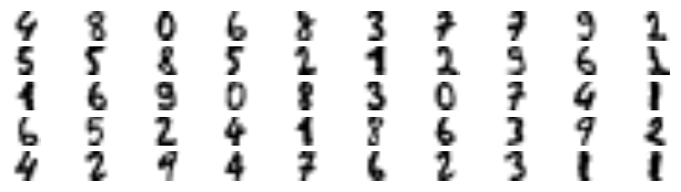
y_train[representative_digit_idx]
array([4, 8, 0, 6, 8, 3, 7, 7, 9, 2, 5, 5, 8, 5, 2, 1, 2, 9, 6, 1, 1, 6,
       9, 0, 8, 3, 0, 7, 4, 1, 6, 5, 2, 4, 1, 8, 6, 3, 9, 2, 4, 2, 9, 4,
       7, 6, 2, 3, 1, 1])
y_representative_digits = np.array([
    0, 1, 3, 2, 7, 6, 4, 6, 9, 5,
    1, 2, 9, 5, 2, 7, 8, 1, 8, 6,
    3, 2, 5, 4, 5, 4, 0, 3, 2, 6,
    1, 7, 7, 9, 1, 8, 6, 5, 4, 8,
    5, 3, 3, 6, 7, 9, 7, 8, 4, 9])
Now we have a dataset with just 50 labeled instances, but instead of being completely random instances, each of them is a representative image of its cluster. Let’s see if the performance is any better:
log_reg = LogisticRegression(multi_class="ovr", solver="lbfgs", max_iter=5000, random_state=42)
log_reg.fit(X_representative_digits, y_representative_digits)
log_reg.score(X_test, y_test)
0.10444444444444445
Wow! We jumped from 83.3% accuracy to 91.3%, although we are still only training the model on 50 instances. Since it’s often costly and painful to label instances, especially when it has to be done manually by experts, it’s a good idea to make them label representative instances rather than just random instances.
But perhaps we can go one step further: what if we propagated the labels to all the other instances in the same cluster?
y_train_propagated = np.empty(len(X_train), dtype=np.int32)
for i in range(k):
    y_train_propagated[kmeans.labels_==i] = y_representative_digits[i]
log_reg = LogisticRegression(multi_class="ovr", solver="lbfgs", max_iter=5000, random_state=42)
log_reg.fit(X_train, y_train_propagated)
LogisticRegression(max_iter=5000, multi_class='ovr', random_state=42)In a Jupyter environment, please rerun this cell to show the HTML representation or trust the notebook.
On GitHub, the HTML representation is unable to render, please try loading this page with nbviewer.org.
LogisticRegression(max_iter=5000, multi_class='ovr', random_state=42)
log_reg.score(X_test, y_test)
0.14888888888888888
We got a tiny little accuracy boost. Better than nothing, but we should probably have propagated the labels only to the instances closest to the centroid, because by propagating to the full cluster, we have certainly included some outliers. Let’s only propagate the labels to the 75th percentile closest to the centroid:
percentile_closest = 75

X_cluster_dist = X_digits_dist[np.arange(len(X_train)), kmeans.labels_]
for i in range(k):
    in_cluster = (kmeans.labels_ == i)
    cluster_dist = X_cluster_dist[in_cluster]
    cutoff_distance = np.percentile(cluster_dist, percentile_closest)
    above_cutoff = (X_cluster_dist > cutoff_distance)
    X_cluster_dist[in_cluster & above_cutoff] = -1
partially_propagated = (X_cluster_dist != -1)
X_train_partially_propagated = X_train[partially_propagated]
y_train_partially_propagated = y_train_propagated[partially_propagated]
log_reg = LogisticRegression(multi_class="ovr", solver="lbfgs", max_iter=5000, random_state=42)
log_reg.fit(X_train_partially_propagated, y_train_partially_propagated)
LogisticRegression(max_iter=5000, multi_class='ovr', random_state=42)In a Jupyter environment, please rerun this cell to show the HTML representation or trust the notebook.
On GitHub, the HTML representation is unable to render, please try loading this page with nbviewer.org.
LogisticRegression(max_iter=5000, multi_class='ovr', random_state=42)
log_reg.score(X_test, y_test)
0.15777777777777777
A bit better. With just 50 labeled instances (just 5 examples per class on average!), we got 92.7% performance, which is getting closer to the performance of logistic regression on the fully labeled digits dataset (which was 96.9%).
This is because the propagated labels are actually pretty good: their accuracy is close to 96%:
np.mean(y_train_partially_propagated == y_train[partially_propagated])
0.19541375872382852
You could now do a few iterations of active learning:
Manually label the instances that the classifier is least sure about, if possible by picking them in distinct clusters.
Train a new model with these additional labels.
17.4. DBSCAN#
from IPython.display import HTML
display(HTML("""
<p style="text-align: center;">
<iframe src="https://static-1300131294.cos.ap-shanghai.myqcloud.com/html/dbscan-demo/dbscan.html" width="105%" height="800px;"
style="border:none;" scrolling="auto"></iframe>
A demo of linear-regression. <a
href="https://www.naftaliharris.com/blog/visualizing-dbscan-clustering/"> [source]</a>
</p>
"""))
A demo of linear-regression. [source]
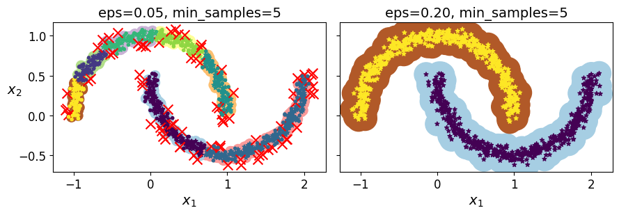
from sklearn.datasets import make_moons
X, y = make_moons(n_samples=1000, noise=0.05, random_state=42)
from sklearn.cluster import DBSCAN
dbscan = DBSCAN(eps=0.05, min_samples=5)
dbscan.fit(X)
DBSCAN(eps=0.05)In a Jupyter environment, please rerun this cell to show the HTML representation or trust the notebook.
On GitHub, the HTML representation is unable to render, please try loading this page with nbviewer.org.
DBSCAN(eps=0.05)
dbscan.labels_[:10]
array([ 0, 2, -1, -1, 1, 0, 0, 0, 2, 5])
len(dbscan.core_sample_indices_)
808
dbscan.core_sample_indices_[:10]
array([ 0, 4, 5, 6, 7, 8, 10, 11, 12, 13])
dbscan.components_[:3]
array([[-0.02137124,  0.40618608],
       [-0.84192557,  0.53058695],
       [ 0.58930337, -0.32137599]])
np.unique(dbscan.labels_)
array([-1, 0, 1, 2, 3, 4, 5, 6])
dbscan2 = DBSCAN(eps=0.2)
dbscan2.fit(X)
DBSCAN(eps=0.2)In a Jupyter environment, please rerun this cell to show the HTML representation or trust the notebook.
On GitHub, the HTML representation is unable to render, please try loading this page with nbviewer.org.
DBSCAN(eps=0.2)
def plot_dbscan(dbscan, X, size, show_xlabels=True, show_ylabels=True):
    core_mask = np.zeros_like(dbscan.labels_, dtype=bool)
    core_mask[dbscan.core_sample_indices_] = True
    anomalies_mask = dbscan.labels_ == -1
    non_core_mask = ~(core_mask | anomalies_mask)

    cores = dbscan.components_
    anomalies = X[anomalies_mask]
    non_cores = X[non_core_mask]

    plt.scatter(cores[:, 0], cores[:, 1],
                c=dbscan.labels_[core_mask], marker='o', s=size, cmap="Paired")
    plt.scatter(cores[:, 0], cores[:, 1], marker='*', s=20, c=dbscan.labels_[core_mask])
    plt.scatter(anomalies[:, 0], anomalies[:, 1],
                c="r", marker="x", s=100)
    plt.scatter(non_cores[:, 0], non_cores[:, 1], c=dbscan.labels_[non_core_mask], marker=".")
    if show_xlabels:
        plt.xlabel("$x_1$", fontsize=14)
    else:
        plt.tick_params(labelbottom=False)
    if show_ylabels:
        plt.ylabel("$x_2$", fontsize=14, rotation=0)
    else:
        plt.tick_params(labelleft=False)
    plt.title("eps={:.2f}, min_samples={}".format(dbscan.eps, dbscan.min_samples), fontsize=14)
plt.figure(figsize=(9, 3.2))

plt.subplot(121)
plot_dbscan(dbscan, X, size=100)

plt.subplot(122)
plot_dbscan(dbscan2, X, size=600, show_ylabels=False)

save_fig("dbscan_plot")
plt.show()
Saving figure dbscan_plot
dbscan = dbscan2
from sklearn.neighbors import KNeighborsClassifier
knn = KNeighborsClassifier(n_neighbors=50)
knn.fit(dbscan.components_, dbscan.labels_[dbscan.core_sample_indices_])
KNeighborsClassifier(n_neighbors=50)In a Jupyter environment, please rerun this cell to show the HTML representation or trust the notebook.
On GitHub, the HTML representation is unable to render, please try loading this page with nbviewer.org.
KNeighborsClassifier(n_neighbors=50)
X_new = np.array([[-0.5, 0], [0, 0.5], [1, -0.1], [2, 1]])
knn.predict(X_new)
array([1, 0, 1, 0])
knn.predict_proba(X_new)
array([[0.18, 0.82],
       [1.  , 0.  ],
       [0.12, 0.88],
       [1.  , 0.  ]])
plt.figure(figsize=(6, 3))
plot_decision_boundaries(knn, X, show_centroids=False)
plt.scatter(X_new[:, 0], X_new[:, 1], c="b", marker="+", s=200, zorder=10)
save_fig("cluster_classification_plot")
plt.show()
Saving figure cluster_classification_plot
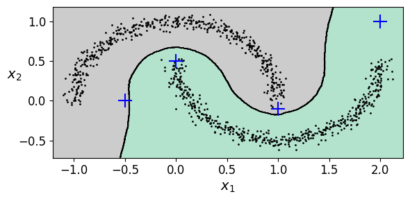
y_dist, y_pred_idx = knn.kneighbors(X_new, n_neighbors=1)
y_pred = dbscan.labels_[dbscan.core_sample_indices_][y_pred_idx]
y_pred[y_dist > 0.2] = -1
y_pred.ravel()
array([-1, 0, 1, -1])
17.5. Hierarchical Clustering#
17.5.1. Spectral Clustering#
from sklearn.cluster import SpectralClustering
sc1 = SpectralClustering(n_clusters=2, gamma=100, random_state=42)
sc1.fit(X)
SpectralClustering(gamma=100, n_clusters=2, random_state=42)In a Jupyter environment, please rerun this cell to show the HTML representation or trust the notebook.
On GitHub, the HTML representation is unable to render, please try loading this page with nbviewer.org.
SpectralClustering(gamma=100, n_clusters=2, random_state=42)
sc2 = SpectralClustering(n_clusters=2, gamma=1, random_state=42)
sc2.fit(X)
SpectralClustering(gamma=1, n_clusters=2, random_state=42)In a Jupyter environment, please rerun this cell to show the HTML representation or trust the notebook.
On GitHub, the HTML representation is unable to render, please try loading this page with nbviewer.org.
SpectralClustering(gamma=1, n_clusters=2, random_state=42)
np.percentile(sc1.affinity_matrix_, 95)
0.04251990648936265
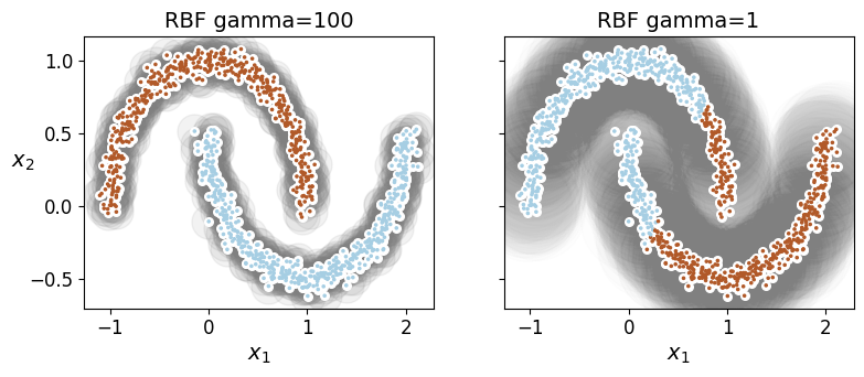
def plot_spectral_clustering(sc, X, size, alpha, show_xlabels=True, show_ylabels=True):
    plt.scatter(X[:, 0], X[:, 1], marker='o', s=size, c='gray', cmap="Paired", alpha=alpha)
    plt.scatter(X[:, 0], X[:, 1], marker='o', s=30, c='w')
    plt.scatter(X[:, 0], X[:, 1], marker='.', s=10, c=sc.labels_, cmap="Paired")

    if show_xlabels:
        plt.xlabel("$x_1$", fontsize=14)
    else:
        plt.tick_params(labelbottom=False)
    if show_ylabels:
        plt.ylabel("$x_2$", fontsize=14, rotation=0)
    else:
        plt.tick_params(labelleft=False)
    plt.title("RBF gamma={}".format(sc.gamma), fontsize=14)
plt.figure(figsize=(9, 3.2))

plt.subplot(121)
plot_spectral_clustering(sc1, X, size=500, alpha=0.1)

plt.subplot(122)
plot_spectral_clustering(sc2, X, size=4000, alpha=0.01, show_ylabels=False)

plt.show()
<ipython-input-127-f4bafb1ea019>:2: UserWarning: No data for colormapping provided via 'c'. Parameters 'cmap' will be ignored
  plt.scatter(X[:, 0], X[:, 1], marker='o', s=size, c='gray', cmap="Paired", alpha=alpha)
17.5.2. Agglomerative Clustering#
from sklearn.cluster import AgglomerativeClustering
X = np.array([0, 2, 5, 8.5]).reshape(-1, 1)
agg = AgglomerativeClustering(linkage="complete").fit(X)
def learned_parameters(estimator):
    return [attrib for attrib in dir(estimator)
            if attrib.endswith("_") and not attrib.startswith("_")]
learned_parameters(agg)
['children_',
 'labels_',
 'n_clusters_',
 'n_connected_components_',
 'n_features_in_',
 'n_leaves_']
agg.children_
array([[0, 1],
       [2, 3],
       [4, 5]])