Bitcoin LSTM Model with Tweet Volume and Sentiment
Contents
42.102. Bitcoin LSTM Model with Tweet Volume and Sentiment#
42.102.1. Load libraries#
import pandas as pd
import re
from matplotlib import pyplot
import seaborn as sns
import numpy as np
import os  # accessing directory structure


# Input data files are available in the "../input/" directory.
# For example, running this (by clicking run or pressing Shift+Enter) will list the files in the input directory

import os

print(os.listdir("/"))

# set seed
np.random.seed(12345)
['$RECYCLE.BIN', '03_IntelliJ IDEA', '2019版安装教程.docx', '46-clion2020破解-无限重置插件', 'Adobe_Premiere Pro 2023', 'anaconda3', 'BaiduNetdisk', 'BaiduNetdiskDownload', 'cent browser', 'CLion 2020.1', 'CLion 2020.1pjb', 'CLionProjects', 'CLIPART', 'CloudMusic', 'CN', 'Config.Msi', 'DAUM', 'Document Themes 16', 'DouyuPCClient', 'DTL8Folder', 'DumpStack.log.tmp', 'Epic Games', 'FFOutput', 'FIRECOLUMN.jpeg', 'FIRECOLUMN1.jpeg', 'FIRECOLUMN2.jpeg', 'firegod.jpg', 'FormatFactory', 'GameDownload', 'Games', 'Git', 'Github', 'GOG Games', 'HuyaClient', 'iGame', 'InfoClient', 'JetBrains', 'kaggle', 'KDR', 'MATLAB_2016', 'Microsoft VS Code', 'MSOCache', 'Netease', 'network', 'Office16', 'Office2016简体中文64位(专业版)', 'opencv', 'pagefile.sys', 'PhotoshopCS6', 'Program Files', 'Program Files (x86)', 'Programs', 'PyCharm 2021.3', 'python', 'qqpcmgr_docpro', 'Recovery', 'Riot Games', 'Stationery', 'steam', 'System Volume Information', 'TECENT_FILES', 'Temp', 'Templates', 'Tencent', 'thunder', 'Thunder.exe', 'Thunder9', 'Tongchuan', 'V2RAYN', 'VSCODEcode', 'WeChat', 'WeChat_Files', 'WECHAT_FILES_COMPUTER', 'yk_temp', 'zd_zts', 'zlad', '斗鱼视频', '新建文件夹', '群星 豪华中文 v3.8.1+银河典范DLC+全DLC+赠品+3.8.2升级补丁 安装即玩', '迅雷云盘', '驱动人生C盘搬家目录']
42.102.2. Data Pre-processing#
notclean = pd.read_csv(
    "https://static-1300131294.cos.ap-shanghai.myqcloud.com/data/deep-learning/LSTM/cleanprep.csv", delimiter=",", on_bad_lines="skip", engine="python", header=None
)
notclean.head()
| 0 | 1 | 2 | 3 | 4 | |
|---|---|---|---|---|---|
| 0 | 2018-07-11 19:35:15.363270 | b'tj' | b"Next two weeks prob v boring (climb up to 9k... | 0.007273 | 0.590909 |
| 1 | 2018-07-11 19:35:15.736769 | b'Kool_Kheart' | b'@Miss_rinola But you\xe2\x80\x99ve heard abo... | 0.000000 | 0.000000 |
| 2 | 2018-07-11 19:35:15.744769 | b'Gary Lang' | b'Duplicate skilled traders automatically with... | 0.625000 | 0.500000 |
| 3 | 2018-07-11 19:35:15.867339 | b'Jobs in Fintech' | b'Project Manager - Technical - FinTech - Cent... | 0.000000 | 0.175000 |
| 4 | 2018-07-11 19:35:16.021448 | b'ERC20' | b'Coinbase App Downloads Drop, Crypto Hype Fad... | 0.333333 | 0.500000 |
# -----------------Pre-processing -------------------#

notclean.columns = ["dt", "name", "text", "polarity", "sensitivity"]
notclean = notclean.drop(["name", "text"], axis=1)
notclean.head()
| dt | polarity | sensitivity | |
|---|---|---|---|
| 0 | 2018-07-11 19:35:15.363270 | 0.007273 | 0.590909 |
| 1 | 2018-07-11 19:35:15.736769 | 0.000000 | 0.000000 |
| 2 | 2018-07-11 19:35:15.744769 | 0.625000 | 0.500000 |
| 3 | 2018-07-11 19:35:15.867339 | 0.000000 | 0.175000 |
| 4 | 2018-07-11 19:35:16.021448 | 0.333333 | 0.500000 |
notclean.info()
<class 'pandas.core.frame.DataFrame'>
RangeIndex: 1413001 entries, 0 to 1413000
Data columns (total 3 columns):
 #   Column       Non-Null Count    Dtype
---  ------       --------------    -----
 0   dt           1413001 non-null  object
 1   polarity     1413001 non-null  float64
 2   sensitivity  1413001 non-null  float64
dtypes: float64(2), object(1)
memory usage: 32.3+ MB
notclean["dt"] = pd.to_datetime(notclean["dt"])
notclean["DateTime"] = notclean["dt"].dt.floor("h")
notclean.head()
| dt | polarity | sensitivity | DateTime | |
|---|---|---|---|---|
| 0 | 2018-07-11 19:35:15.363270 | 0.007273 | 0.590909 | 2018-07-11 19:00:00 |
| 1 | 2018-07-11 19:35:15.736769 | 0.000000 | 0.000000 | 2018-07-11 19:00:00 |
| 2 | 2018-07-11 19:35:15.744769 | 0.625000 | 0.500000 | 2018-07-11 19:00:00 |
| 3 | 2018-07-11 19:35:15.867339 | 0.000000 | 0.175000 | 2018-07-11 19:00:00 |
| 4 | 2018-07-11 19:35:16.021448 | 0.333333 | 0.500000 | 2018-07-11 19:00:00 |
vdf = (
    notclean.groupby(pd.Grouper(key="dt", freq="H"))
    .size()
    .reset_index(name="tweet_vol")
)
vdf.head()
| dt | tweet_vol | |
|---|---|---|
| 0 | 2018-07-11 19:00:00 | 1747 |
| 1 | 2018-07-11 20:00:00 | 4354 |
| 2 | 2018-07-11 21:00:00 | 4432 |
| 3 | 2018-07-11 22:00:00 | 3980 |
| 4 | 2018-07-11 23:00:00 | 3830 |
vdf.info()
<class 'pandas.core.frame.DataFrame'>
RangeIndex: 302 entries, 0 to 301
Data columns (total 2 columns):
 #   Column     Non-Null Count  Dtype
---  ------     --------------  -----
 0   dt         302 non-null    datetime64[ns]
 1   tweet_vol  302 non-null    int64
dtypes: datetime64[ns](1), int64(1)
memory usage: 4.8 KB
vdf.index = pd.to_datetime(vdf.index)
vdf = vdf.set_index("dt")
vdf.info()
<class 'pandas.core.frame.DataFrame'>
DatetimeIndex: 302 entries, 2018-07-11 19:00:00 to 2018-07-24 08:00:00
Data columns (total 1 columns):
 #   Column     Non-Null Count  Dtype
---  ------     --------------  -----
 0   tweet_vol  302 non-null    int64
dtypes: int64(1)
memory usage: 4.7 KB
vdf.head()
| tweet_vol | |
|---|---|
| dt | |
| 2018-07-11 19:00:00 | 1747 |
| 2018-07-11 20:00:00 | 4354 |
| 2018-07-11 21:00:00 | 4432 |
| 2018-07-11 22:00:00 | 3980 |
| 2018-07-11 23:00:00 | 3830 |
notclean.info()
<class 'pandas.core.frame.DataFrame'>
RangeIndex: 1413001 entries, 0 to 1413000
Data columns (total 4 columns):
 #   Column       Non-Null Count    Dtype
---  ------       --------------    -----
 0   dt           1413001 non-null  datetime64[ns]
 1   polarity     1413001 non-null  float64
 2   sensitivity  1413001 non-null  float64
 3   DateTime     1413001 non-null  datetime64[ns]
dtypes: datetime64[ns](2), float64(2)
memory usage: 43.1 MB
notclean.index = pd.to_datetime(notclean.index)
notclean.info()
<class 'pandas.core.frame.DataFrame'>
DatetimeIndex: 1413001 entries, 1970-01-01 00:00:00 to 1970-01-01 00:00:00.001413
Data columns (total 4 columns):
 #   Column       Non-Null Count    Dtype
---  ------       --------------    -----
 0   dt           1413001 non-null  datetime64[ns]
 1   polarity     1413001 non-null  float64
 2   sensitivity  1413001 non-null  float64
 3   DateTime     1413001 non-null  datetime64[ns]
dtypes: datetime64[ns](2), float64(2)
memory usage: 53.9 MB
vdf["tweet_vol"] = vdf["tweet_vol"].astype(float)
vdf.info()
<class 'pandas.core.frame.DataFrame'>
DatetimeIndex: 302 entries, 2018-07-11 19:00:00 to 2018-07-24 08:00:00
Data columns (total 1 columns):
 #   Column     Non-Null Count  Dtype
---  ------     --------------  -----
 0   tweet_vol  302 non-null    float64
dtypes: float64(1)
memory usage: 4.7 KB
notclean.info()
<class 'pandas.core.frame.DataFrame'>
DatetimeIndex: 1413001 entries, 1970-01-01 00:00:00 to 1970-01-01 00:00:00.001413
Data columns (total 4 columns):
 #   Column       Non-Null Count    Dtype
---  ------       --------------    -----
 0   dt           1413001 non-null  datetime64[ns]
 1   polarity     1413001 non-null  float64
 2   sensitivity  1413001 non-null  float64
 3   DateTime     1413001 non-null  datetime64[ns]
dtypes: datetime64[ns](2), float64(2)
memory usage: 53.9 MB
notclean.head()
| dt | polarity | sensitivity | DateTime | |
|---|---|---|---|---|
| 1970-01-01 00:00:00.000000000 | 2018-07-11 19:35:15.363270 | 0.007273 | 0.590909 | 2018-07-11 19:00:00 |
| 1970-01-01 00:00:00.000000001 | 2018-07-11 19:35:15.736769 | 0.000000 | 0.000000 | 2018-07-11 19:00:00 |
| 1970-01-01 00:00:00.000000002 | 2018-07-11 19:35:15.744769 | 0.625000 | 0.500000 | 2018-07-11 19:00:00 |
| 1970-01-01 00:00:00.000000003 | 2018-07-11 19:35:15.867339 | 0.000000 | 0.175000 | 2018-07-11 19:00:00 |
| 1970-01-01 00:00:00.000000004 | 2018-07-11 19:35:16.021448 | 0.333333 | 0.500000 | 2018-07-11 19:00:00 |
# ndf = pd.merge(notclean,vdf, how='inner',left_index=True, right_index=True)
notclean.head()
| dt | polarity | sensitivity | DateTime | |
|---|---|---|---|---|
| 1970-01-01 00:00:00.000000000 | 2018-07-11 19:35:15.363270 | 0.007273 | 0.590909 | 2018-07-11 19:00:00 |
| 1970-01-01 00:00:00.000000001 | 2018-07-11 19:35:15.736769 | 0.000000 | 0.000000 | 2018-07-11 19:00:00 |
| 1970-01-01 00:00:00.000000002 | 2018-07-11 19:35:15.744769 | 0.625000 | 0.500000 | 2018-07-11 19:00:00 |
| 1970-01-01 00:00:00.000000003 | 2018-07-11 19:35:15.867339 | 0.000000 | 0.175000 | 2018-07-11 19:00:00 |
| 1970-01-01 00:00:00.000000004 | 2018-07-11 19:35:16.021448 | 0.333333 | 0.500000 | 2018-07-11 19:00:00 |
df = notclean.groupby("DateTime").agg(lambda x: x.mean())
df["Tweet_vol"] = vdf["tweet_vol"]
df = df.drop(df.index[0])
df.head()
| dt | polarity | sensitivity | Tweet_vol | |
|---|---|---|---|---|
| DateTime | ||||
| 2018-07-11 20:00:00 | 2018-07-11 20:27:49.510636288 | 0.102657 | 0.216148 | 4354.0 |
| 2018-07-11 21:00:00 | 2018-07-11 21:28:35.636368640 | 0.098004 | 0.218612 | 4432.0 |
| 2018-07-11 22:00:00 | 2018-07-11 22:27:44.646705152 | 0.096688 | 0.231342 | 3980.0 |
| 2018-07-11 23:00:00 | 2018-07-11 23:28:06.455850496 | 0.103997 | 0.217739 | 3830.0 |
| 2018-07-12 00:00:00 | 2018-07-12 00:28:47.975385344 | 0.094383 | 0.195256 | 3998.0 |
df.tail()
| dt | polarity | sensitivity | Tweet_vol | |
|---|---|---|---|---|
| DateTime | ||||
| 2018-07-24 04:00:00 | 2018-07-24 04:27:40.946246656 | 0.121358 | 0.236000 | 4475.0 |
| 2018-07-24 05:00:00 | 2018-07-24 05:28:40.424965632 | 0.095163 | 0.216924 | 4808.0 |
| 2018-07-24 06:00:00 | 2018-07-24 06:30:52.606722816 | 0.088992 | 0.220173 | 6036.0 |
| 2018-07-24 07:00:00 | 2018-07-24 07:27:29.229673984 | 0.091439 | 0.198279 | 6047.0 |
| 2018-07-24 08:00:00 | 2018-07-24 08:07:02.674452224 | 0.071268 | 0.218217 | 2444.0 |
df.info()
<class 'pandas.core.frame.DataFrame'>
DatetimeIndex: 301 entries, 2018-07-11 20:00:00 to 2018-07-24 08:00:00
Data columns (total 4 columns):
 #   Column       Non-Null Count  Dtype
---  ------       --------------  -----
 0   dt           301 non-null    datetime64[ns]
 1   polarity     301 non-null    float64
 2   sensitivity  301 non-null    float64
 3   Tweet_vol    301 non-null    float64
dtypes: datetime64[ns](1), float64(3)
memory usage: 11.8 KB
btcDF = pd.read_csv("https://static-1300131294.cos.ap-shanghai.myqcloud.com/data/deep-learning/LSTM/btcSave2.csv", on_bad_lines="skip", engine="python")
btcDF["Timestamp"] = pd.to_datetime(btcDF["Timestamp"])
btcDF = btcDF.set_index(pd.DatetimeIndex(btcDF["Timestamp"]))
btcDF.head()
| Timestamp | Open | High | Low | Close | Volume (BTC) | Volume (Currency) | Weighted Price | |
|---|---|---|---|---|---|---|---|---|
| Timestamp | ||||||||
| 2018-07-10 01:00:00 | 2018-07-10 01:00:00 | 6666.75 | 6683.90 | 6635.59 | 6669.73 | 281.73 | 1875693.72 | 6657.70 |
| 2018-07-10 02:00:00 | 2018-07-10 02:00:00 | 6662.44 | 6674.60 | 6647.00 | 6647.00 | 174.10 | 1160103.29 | 6663.38 |
| 2018-07-10 03:00:00 | 2018-07-10 03:00:00 | 6652.52 | 6662.82 | 6621.99 | 6632.53 | 231.41 | 1536936.22 | 6641.70 |
| 2018-07-10 04:00:00 | 2018-07-10 04:00:00 | 6631.17 | 6655.48 | 6625.54 | 6635.92 | 120.38 | 799154.77 | 6638.52 |
| 2018-07-10 05:00:00 | 2018-07-10 05:00:00 | 6632.81 | 6651.06 | 6627.64 | 6640.57 | 94.00 | 624289.31 | 6641.32 |
btcDF = btcDF.drop(["Timestamp"], axis=1)
btcDF.head()
| Open | High | Low | Close | Volume (BTC) | Volume (Currency) | Weighted Price | |
|---|---|---|---|---|---|---|---|
| Timestamp | |||||||
| 2018-07-10 01:00:00 | 6666.75 | 6683.90 | 6635.59 | 6669.73 | 281.73 | 1875693.72 | 6657.70 |
| 2018-07-10 02:00:00 | 6662.44 | 6674.60 | 6647.00 | 6647.00 | 174.10 | 1160103.29 | 6663.38 |
| 2018-07-10 03:00:00 | 6652.52 | 6662.82 | 6621.99 | 6632.53 | 231.41 | 1536936.22 | 6641.70 |
| 2018-07-10 04:00:00 | 6631.17 | 6655.48 | 6625.54 | 6635.92 | 120.38 | 799154.77 | 6638.52 |
| 2018-07-10 05:00:00 | 6632.81 | 6651.06 | 6627.64 | 6640.57 | 94.00 | 624289.31 | 6641.32 |
Final_df = pd.merge(df, btcDF, how="inner", left_index=True, right_index=True)
Final_df.head()
| dt | polarity | sensitivity | Tweet_vol | Open | High | Low | Close | Volume (BTC) | Volume (Currency) | Weighted Price | |
|---|---|---|---|---|---|---|---|---|---|---|---|
| 2018-07-11 20:00:00 | 2018-07-11 20:27:49.510636288 | 0.102657 | 0.216148 | 4354.0 | 6342.97 | 6354.19 | 6291.00 | 6350.00 | 986.73 | 6231532.37 | 6315.33 |
| 2018-07-11 21:00:00 | 2018-07-11 21:28:35.636368640 | 0.098004 | 0.218612 | 4432.0 | 6352.99 | 6370.00 | 6345.76 | 6356.48 | 126.46 | 804221.55 | 6359.53 |
| 2018-07-11 22:00:00 | 2018-07-11 22:27:44.646705152 | 0.096688 | 0.231342 | 3980.0 | 6350.85 | 6378.47 | 6345.00 | 6361.93 | 259.10 | 1646353.87 | 6354.12 |
| 2018-07-11 23:00:00 | 2018-07-11 23:28:06.455850496 | 0.103997 | 0.217739 | 3830.0 | 6362.36 | 6381.25 | 6356.74 | 6368.78 | 81.54 | 519278.69 | 6368.23 |
| 2018-07-12 00:00:00 | 2018-07-12 00:28:47.975385344 | 0.094383 | 0.195256 | 3998.0 | 6369.49 | 6381.25 | 6361.83 | 6380.00 | 124.55 | 793560.22 | 6371.51 |
Final_df.info()
<class 'pandas.core.frame.DataFrame'>
DatetimeIndex: 294 entries, 2018-07-11 20:00:00 to 2018-07-24 01:00:00
Data columns (total 11 columns):
 #   Column             Non-Null Count  Dtype
---  ------             --------------  -----
 0   dt                 294 non-null    datetime64[ns]
 1   polarity           294 non-null    float64
 2   sensitivity        294 non-null    float64
 3   Tweet_vol          294 non-null    float64
 4   Open               294 non-null    float64
 5   High               294 non-null    float64
 6   Low                294 non-null    float64
 7   Close              294 non-null    float64
 8   Volume (BTC)       294 non-null    float64
 9   Volume (Currency)  294 non-null    float64
 10  Weighted Price     294 non-null    float64
dtypes: datetime64[ns](1), float64(10)
memory usage: 27.6 KB
Final_df = Final_df.drop(["Weighted Price"], axis=1)
Final_df.head()
| dt | polarity | sensitivity | Tweet_vol | Open | High | Low | Close | Volume (BTC) | Volume (Currency) | |
|---|---|---|---|---|---|---|---|---|---|---|
| 2018-07-11 20:00:00 | 2018-07-11 20:27:49.510636288 | 0.102657 | 0.216148 | 4354.0 | 6342.97 | 6354.19 | 6291.00 | 6350.00 | 986.73 | 6231532.37 |
| 2018-07-11 21:00:00 | 2018-07-11 21:28:35.636368640 | 0.098004 | 0.218612 | 4432.0 | 6352.99 | 6370.00 | 6345.76 | 6356.48 | 126.46 | 804221.55 |
| 2018-07-11 22:00:00 | 2018-07-11 22:27:44.646705152 | 0.096688 | 0.231342 | 3980.0 | 6350.85 | 6378.47 | 6345.00 | 6361.93 | 259.10 | 1646353.87 |
| 2018-07-11 23:00:00 | 2018-07-11 23:28:06.455850496 | 0.103997 | 0.217739 | 3830.0 | 6362.36 | 6381.25 | 6356.74 | 6368.78 | 81.54 | 519278.69 |
| 2018-07-12 00:00:00 | 2018-07-12 00:28:47.975385344 | 0.094383 | 0.195256 | 3998.0 | 6369.49 | 6381.25 | 6361.83 | 6380.00 | 124.55 | 793560.22 |
Final_df.columns = [
    "dt",
    "Polarity",
    "Sensitivity",
    "Tweet_vol",
    "Open",
    "High",
    "Low",
    "Close_Price",
    "Volume_BTC",
    "Volume_Dollar",
]
Final_df.head()
| dt | Polarity | Sensitivity | Tweet_vol | Open | High | Low | Close_Price | Volume_BTC | Volume_Dollar | |
|---|---|---|---|---|---|---|---|---|---|---|
| 2018-07-11 20:00:00 | 2018-07-11 20:27:49.510636288 | 0.102657 | 0.216148 | 4354.0 | 6342.97 | 6354.19 | 6291.00 | 6350.00 | 986.73 | 6231532.37 |
| 2018-07-11 21:00:00 | 2018-07-11 21:28:35.636368640 | 0.098004 | 0.218612 | 4432.0 | 6352.99 | 6370.00 | 6345.76 | 6356.48 | 126.46 | 804221.55 |
| 2018-07-11 22:00:00 | 2018-07-11 22:27:44.646705152 | 0.096688 | 0.231342 | 3980.0 | 6350.85 | 6378.47 | 6345.00 | 6361.93 | 259.10 | 1646353.87 |
| 2018-07-11 23:00:00 | 2018-07-11 23:28:06.455850496 | 0.103997 | 0.217739 | 3830.0 | 6362.36 | 6381.25 | 6356.74 | 6368.78 | 81.54 | 519278.69 |
| 2018-07-12 00:00:00 | 2018-07-12 00:28:47.975385344 | 0.094383 | 0.195256 | 3998.0 | 6369.49 | 6381.25 | 6361.83 | 6380.00 | 124.55 | 793560.22 |
Final_df = Final_df[
    [
        "Polarity",
        "Sensitivity",
        "Tweet_vol",
        "Open",
        "High",
        "Low",
        "Volume_BTC",
        "Volume_Dollar",
        "Close_Price",
    ]
]
Final_df
| Polarity | Sensitivity | Tweet_vol | Open | High | Low | Volume_BTC | Volume_Dollar | Close_Price | |
|---|---|---|---|---|---|---|---|---|---|
| 2018-07-11 20:00:00 | 0.102657 | 0.216148 | 4354.0 | 6342.97 | 6354.19 | 6291.00 | 986.73 | 6231532.37 | 6350.00 |
| 2018-07-11 21:00:00 | 0.098004 | 0.218612 | 4432.0 | 6352.99 | 6370.00 | 6345.76 | 126.46 | 804221.55 | 6356.48 |
| 2018-07-11 22:00:00 | 0.096688 | 0.231342 | 3980.0 | 6350.85 | 6378.47 | 6345.00 | 259.10 | 1646353.87 | 6361.93 |
| 2018-07-11 23:00:00 | 0.103997 | 0.217739 | 3830.0 | 6362.36 | 6381.25 | 6356.74 | 81.54 | 519278.69 | 6368.78 |
| 2018-07-12 00:00:00 | 0.094383 | 0.195256 | 3998.0 | 6369.49 | 6381.25 | 6361.83 | 124.55 | 793560.22 | 6380.00 |
| ... | ... | ... | ... | ... | ... | ... | ... | ... | ... |
| 2018-07-23 21:00:00 | 0.107282 | 0.235636 | 5164.0 | 7746.99 | 7763.59 | 7690.16 | 237.63 | 1836633.86 | 7706.00 |
| 2018-07-23 22:00:00 | 0.094493 | 0.271796 | 4646.0 | 7699.13 | 7759.99 | 7690.50 | 63.31 | 489000.25 | 7750.09 |
| 2018-07-23 23:00:00 | 0.074246 | 0.231640 | 4455.0 | 7754.57 | 7777.00 | 7715.45 | 280.46 | 2173424.81 | 7722.32 |
| 2018-07-24 00:00:00 | 0.080870 | 0.219367 | 3862.0 | 7722.95 | 7730.61 | 7690.17 | 496.48 | 3830571.66 | 7719.62 |
| 2018-07-24 01:00:00 | 0.090717 | 0.212626 | 4620.0 | 7712.46 | 7727.70 | 7691.14 | 163.99 | 1264085.79 | 7723.22 |
294 rows × 9 columns
42.102.3. Exploratory Analysis#
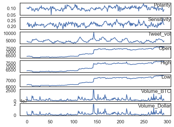
# --------------Analysis----------------------------#

values = Final_df.values
groups = [0, 1, 2, 3, 4, 5, 6, 7]
i = 1
pyplot.figure()
for group in groups:
    pyplot.subplot(len(groups), 1, i)
    pyplot.plot(values[:, group])
    pyplot.title(Final_df.columns[group], y=0.5, loc="right")
    i += 1
pyplot.show()
Final_df["Volume_BTC"].max()
2640.49
Final_df["Volume_Dollar"].max()
19126407.89
Final_df["Volume_BTC"].sum()
96945.04000000001
Final_df["Volume_Dollar"].sum()
684457140.05
Final_df["Tweet_vol"].max()
10452.0
Final_df.describe()
| Polarity | Sensitivity | Tweet_vol | Open | High | Low | Volume_BTC | Volume_Dollar | Close_Price | |
|---|---|---|---|---|---|---|---|---|---|
| count | 294.000000 | 294.000000 | 294.000000 | 294.000000 | 294.000000 | 294.000000 | 294.000000 | 2.940000e+02 | 294.000000 |
| mean | 0.099534 | 0.214141 | 4691.119048 | 6915.349388 | 6946.782925 | 6889.661054 | 329.745034 | 2.328086e+06 | 6920.150000 |
| std | 0.012114 | 0.014940 | 1048.922706 | 564.467674 | 573.078843 | 559.037540 | 344.527625 | 2.508128e+06 | 565.424866 |
| min | 0.051695 | 0.174330 | 2998.000000 | 6149.110000 | 6173.610000 | 6072.000000 | 22.000000 | 1.379601e+05 | 6149.110000 |
| 25% | 0.091489 | 0.203450 | 3878.750000 | 6285.077500 | 6334.942500 | 6266.522500 | 129.230000 | 8.412214e+05 | 6283.497500 |
| 50% | 0.099198 | 0.214756 | 4452.000000 | 7276.845000 | 7311.380000 | 7245.580000 | 223.870000 | 1.607008e+06 | 7281.975000 |
| 75% | 0.106649 | 0.223910 | 5429.750000 | 7422.957500 | 7457.202500 | 7396.427500 | 385.135000 | 2.662185e+06 | 7424.560000 |
| max | 0.135088 | 0.271796 | 10452.000000 | 7754.570000 | 7800.000000 | 7724.500000 | 2640.490000 | 1.912641e+07 | 7750.090000 |
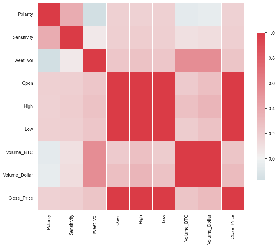
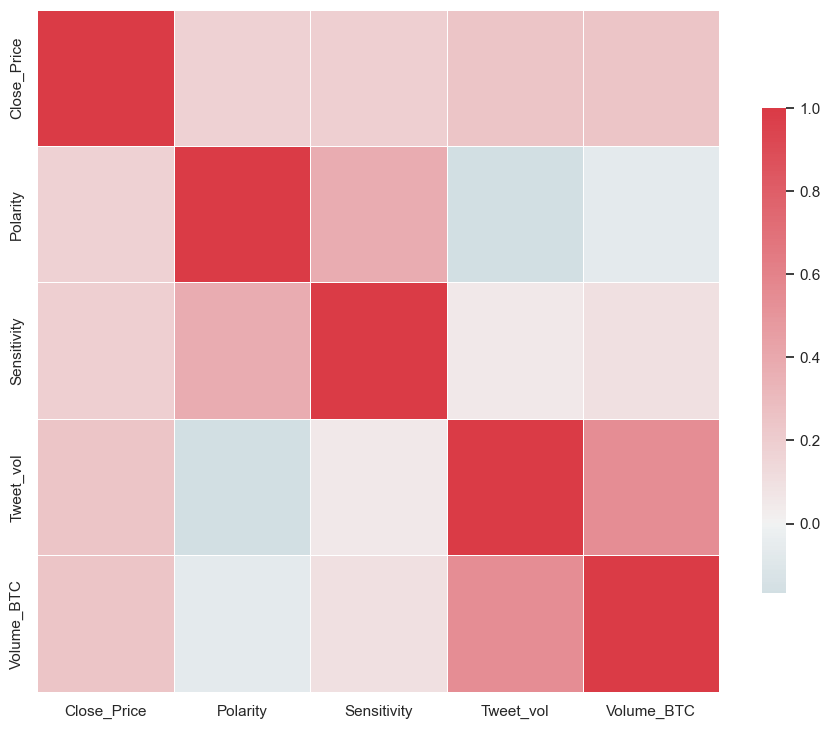
cor = Final_df.corr()
cor
| Polarity | Sensitivity | Tweet_vol | Open | High | Low | Volume_BTC | Volume_Dollar | Close_Price | |
|---|---|---|---|---|---|---|---|---|---|
| Polarity | 1.000000 | 0.380350 | -0.167573 | 0.179056 | 0.176277 | 0.180088 | -0.062868 | -0.052646 | 0.178456 |
| Sensitivity | 0.380350 | 1.000000 | 0.053903 | 0.194763 | 0.200611 | 0.190222 | 0.097124 | 0.112425 | 0.193203 |
| Tweet_vol | -0.167573 | 0.053903 | 1.000000 | 0.237185 | 0.262207 | 0.234330 | 0.541112 | 0.545850 | 0.250448 |
| Open | 0.179056 | 0.194763 | 0.237185 | 1.000000 | 0.997128 | 0.998799 | 0.217478 | 0.277600 | 0.997217 |
| High | 0.176277 | 0.200611 | 0.262207 | 0.997128 | 1.000000 | 0.996650 | 0.270551 | 0.329816 | 0.998816 |
| Low | 0.180088 | 0.190222 | 0.234330 | 0.998799 | 0.996650 | 1.000000 | 0.202895 | 0.263863 | 0.998058 |
| Volume_BTC | -0.062868 | 0.097124 | 0.541112 | 0.217478 | 0.270551 | 0.202895 | 1.000000 | 0.995873 | 0.243875 |
| Volume_Dollar | -0.052646 | 0.112425 | 0.545850 | 0.277600 | 0.329816 | 0.263863 | 0.995873 | 1.000000 | 0.303347 |
| Close_Price | 0.178456 | 0.193203 | 0.250448 | 0.997217 | 0.998816 | 0.998058 | 0.243875 | 0.303347 | 1.000000 |
Top_Vol = Final_df["Volume_BTC"].nlargest(10)
Top_Vol
2018-07-17 18:00:00    2640.49
2018-07-17 19:00:00    2600.32
2018-07-23 03:00:00    1669.28
2018-07-18 04:00:00    1576.15
2018-07-20 17:00:00    1510.00
2018-07-18 19:00:00    1490.02
2018-07-23 19:00:00    1396.32
2018-07-12 07:00:00    1211.64
2018-07-16 10:00:00    1147.69
2018-07-23 08:00:00    1135.38
Name: Volume_BTC, dtype: float64
Top_Sen = Final_df["Sensitivity"].nlargest(10)
Top_Sen
2018-07-23 22:00:00    0.271796
2018-07-19 20:00:00    0.262048
2018-07-21 19:00:00    0.256952
2018-07-20 22:00:00    0.246046
2018-07-22 06:00:00    0.245820
2018-07-19 19:00:00    0.244655
2018-07-19 21:00:00    0.244215
2018-07-18 20:00:00    0.243534
2018-07-18 21:00:00    0.243422
2018-07-18 18:00:00    0.241287
Name: Sensitivity, dtype: float64
Top_Pol = Final_df["Polarity"].nlargest(10)
Top_Pol
2018-07-22 05:00:00    0.135088
2018-07-16 03:00:00    0.130634
2018-07-19 20:00:00    0.127696
2018-07-15 10:00:00    0.127469
2018-07-22 06:00:00    0.126299
2018-07-15 06:00:00    0.124505
2018-07-16 05:00:00    0.124210
2018-07-22 09:00:00    0.122784
2018-07-15 13:00:00    0.122411
2018-07-22 12:00:00    0.122021
Name: Polarity, dtype: float64
Top_Tweet = Final_df["Tweet_vol"].nlargest(10)
Top_Tweet
2018-07-17 19:00:00    10452.0
2018-07-17 18:00:00     7995.0
2018-07-17 20:00:00     7354.0
2018-07-16 14:00:00     7280.0
2018-07-18 15:00:00     7222.0
2018-07-18 14:00:00     7209.0
2018-07-18 13:00:00     7171.0
2018-07-16 13:00:00     7133.0
2018-07-19 16:00:00     6886.0
2018-07-18 12:00:00     6844.0
Name: Tweet_vol, dtype: float64
import matplotlib.pyplot as plt

sns.set(style="white")
f, ax = plt.subplots(figsize=(11, 9))

cmap = sns.diverging_palette(220, 10, as_cmap=True)
ax = sns.heatmap(
    cor,
    cmap=cmap,
    vmax=1,
    center=0,
    square=True,
    linewidths=0.5,
    cbar_kws={"shrink": 0.7},
)
plt.show()
# sns Heatmap for Hour x volume
# Final_df['time']=Final_df.index.time()
Final_df["time"] = Final_df.index.to_series().apply(lambda x: x.strftime("%X"))
Final_df.head()
| Polarity | Sensitivity | Tweet_vol | Open | High | Low | Volume_BTC | Volume_Dollar | Close_Price | time | |
|---|---|---|---|---|---|---|---|---|---|---|
| 2018-07-11 20:00:00 | 0.102657 | 0.216148 | 4354.0 | 6342.97 | 6354.19 | 6291.00 | 986.73 | 6231532.37 | 6350.00 | 20:00:00 |
| 2018-07-11 21:00:00 | 0.098004 | 0.218612 | 4432.0 | 6352.99 | 6370.00 | 6345.76 | 126.46 | 804221.55 | 6356.48 | 21:00:00 |
| 2018-07-11 22:00:00 | 0.096688 | 0.231342 | 3980.0 | 6350.85 | 6378.47 | 6345.00 | 259.10 | 1646353.87 | 6361.93 | 22:00:00 |
| 2018-07-11 23:00:00 | 0.103997 | 0.217739 | 3830.0 | 6362.36 | 6381.25 | 6356.74 | 81.54 | 519278.69 | 6368.78 | 23:00:00 |
| 2018-07-12 00:00:00 | 0.094383 | 0.195256 | 3998.0 | 6369.49 | 6381.25 | 6361.83 | 124.55 | 793560.22 | 6380.00 | 00:00:00 |
hour_df = Final_df
hour_df = hour_df.groupby("time").agg(lambda x: x.mean())
hour_df
| Polarity | Sensitivity | Tweet_vol | Open | High | Low | Volume_BTC | Volume_Dollar | Close_Price | |
|---|---|---|---|---|---|---|---|---|---|
| time | |||||||||
| 00:00:00 | 0.090298 | 0.211771 | 3976.384615 | 6930.237692 | 6958.360769 | 6900.588462 | 322.836154 | 2.228120e+06 | 6935.983077 |
| 01:00:00 | 0.099596 | 0.211714 | 4016.615385 | 6935.140769 | 6963.533846 | 6894.772308 | 318.415385 | 2.243338e+06 | 6933.794615 |
| 02:00:00 | 0.102724 | 0.204445 | 3824.083333 | 6868.211667 | 6889.440000 | 6842.588333 | 158.836667 | 1.105651e+06 | 6870.695833 |
| 03:00:00 | 0.105586 | 0.214824 | 3791.666667 | 6870.573333 | 6909.675833 | 6855.316667 | 328.811667 | 2.385733e+06 | 6888.139167 |
| 04:00:00 | 0.103095 | 0.208516 | 3822.916667 | 6887.420000 | 6911.649167 | 6872.603333 | 271.692500 | 1.949230e+06 | 6890.985000 |
| 05:00:00 | 0.108032 | 0.215058 | 3904.166667 | 6891.468333 | 6911.175833 | 6869.017500 | 213.315000 | 1.524601e+06 | 6890.451667 |
| 06:00:00 | 0.104412 | 0.210424 | 3760.250000 | 6889.327500 | 6907.070833 | 6868.484167 | 183.329167 | 1.281427e+06 | 6891.371667 |
| 07:00:00 | 0.100942 | 0.209435 | 4056.000000 | 6891.645833 | 6908.654167 | 6858.290833 | 329.882500 | 2.263694e+06 | 6878.757500 |
| 08:00:00 | 0.099380 | 0.210113 | 5095.583333 | 6878.635833 | 6903.660833 | 6851.435833 | 368.109167 | 2.616314e+06 | 6885.867500 |
| 09:00:00 | 0.099369 | 0.204565 | 4650.083333 | 6886.526667 | 6915.735000 | 6852.922500 | 397.702500 | 2.740251e+06 | 6888.328333 |
| 10:00:00 | 0.099587 | 0.203848 | 4932.833333 | 6888.095000 | 6921.905000 | 6870.502500 | 318.982500 | 2.194532e+06 | 6905.600833 |
| 11:00:00 | 0.097061 | 0.203488 | 4996.333333 | 6904.373333 | 6928.490000 | 6885.326667 | 256.131667 | 1.766995e+06 | 6907.590000 |
| 12:00:00 | 0.099139 | 0.207495 | 5446.583333 | 6908.016667 | 6942.194167 | 6890.370000 | 314.837500 | 2.200126e+06 | 6922.389167 |
| 13:00:00 | 0.097565 | 0.208969 | 5565.083333 | 6922.530000 | 6948.463333 | 6902.968333 | 260.825000 | 1.808326e+06 | 6925.079167 |
| 14:00:00 | 0.098485 | 0.212563 | 5736.583333 | 6925.589167 | 6952.400833 | 6908.944167 | 288.322500 | 2.033892e+06 | 6936.545833 |
| 15:00:00 | 0.099428 | 0.212782 | 5686.500000 | 6934.180833 | 6965.962500 | 6915.395833 | 326.230000 | 2.313765e+06 | 6937.513333 |
| 16:00:00 | 0.098327 | 0.215643 | 5647.250000 | 6937.987500 | 6970.406667 | 6914.132500 | 411.930833 | 2.977255e+06 | 6947.045000 |
| 17:00:00 | 0.099674 | 0.219544 | 5482.333333 | 6947.205000 | 6986.905000 | 6928.375833 | 421.290833 | 3.020724e+06 | 6946.573333 |
| 18:00:00 | 0.098512 | 0.223854 | 5340.666667 | 6946.270833 | 7020.676667 | 6917.940000 | 621.599167 | 4.405309e+06 | 6985.155833 |
| 19:00:00 | 0.094025 | 0.227546 | 5345.583333 | 6984.812500 | 7048.856667 | 6948.802500 | 635.320833 | 4.639426e+06 | 6990.852500 |
| 20:00:00 | 0.096545 | 0.221846 | 4829.692308 | 6941.196923 | 6968.019231 | 6903.869231 | 396.382308 | 2.764029e+06 | 6937.162308 |
| 21:00:00 | 0.100486 | 0.227031 | 4586.076923 | 6937.536923 | 6961.624615 | 6902.450000 | 320.918462 | 2.235449e+06 | 6929.238462 |
| 22:00:00 | 0.101451 | 0.231768 | 4215.769231 | 6928.340769 | 6960.293846 | 6899.097692 | 201.525385 | 1.425684e+06 | 6924.276923 |
| 23:00:00 | 0.096164 | 0.218966 | 4081.230769 | 6924.337692 | 6960.037692 | 6893.017692 | 259.863846 | 1.851852e+06 | 6928.529231 |
hour_df.head()
| Polarity | Sensitivity | Tweet_vol | Open | High | Low | Volume_BTC | Volume_Dollar | Close_Price | |
|---|---|---|---|---|---|---|---|---|---|
| time | |||||||||
| 00:00:00 | 0.090298 | 0.211771 | 3976.384615 | 6930.237692 | 6958.360769 | 6900.588462 | 322.836154 | 2.228120e+06 | 6935.983077 |
| 01:00:00 | 0.099596 | 0.211714 | 4016.615385 | 6935.140769 | 6963.533846 | 6894.772308 | 318.415385 | 2.243338e+06 | 6933.794615 |
| 02:00:00 | 0.102724 | 0.204445 | 3824.083333 | 6868.211667 | 6889.440000 | 6842.588333 | 158.836667 | 1.105651e+06 | 6870.695833 |
| 03:00:00 | 0.105586 | 0.214824 | 3791.666667 | 6870.573333 | 6909.675833 | 6855.316667 | 328.811667 | 2.385733e+06 | 6888.139167 |
| 04:00:00 | 0.103095 | 0.208516 | 3822.916667 | 6887.420000 | 6911.649167 | 6872.603333 | 271.692500 | 1.949230e+06 | 6890.985000 |
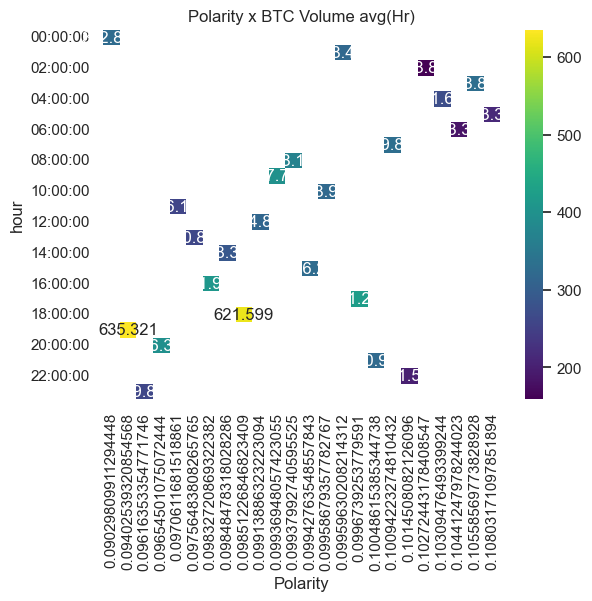
# sns Hourly Heatmap
hour_df["hour"] = hour_df.index
result = hour_df.pivot(index="hour", columns="Polarity", values="Volume_BTC")
sns.heatmap(result, annot=True, fmt="g", cmap="viridis")
plt.title("Polarity x BTC Volume avg(Hr)")
plt.show()
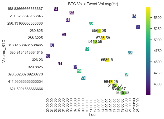
# sns daily heatmap?
hour_df["hour"] = hour_df.index
result = hour_df.pivot(index="Volume_BTC", columns="hour", values="Tweet_vol")
sns.heatmap(result, annot=True, fmt="g", cmap="viridis")
plt.title("BTC Vol x Tweet Vol avg(Hr)")
plt.show()
# ----------------End Analysis------------------------#
# ---------------- LSTM Prep ------------------------#
df = Final_df
df.info()
<class 'pandas.core.frame.DataFrame'>
DatetimeIndex: 294 entries, 2018-07-11 20:00:00 to 2018-07-24 01:00:00
Data columns (total 10 columns):
 #   Column         Non-Null Count  Dtype
---  ------         --------------  -----
 0   Polarity       294 non-null    float64
 1   Sensitivity    294 non-null    float64
 2   Tweet_vol      294 non-null    float64
 3   Open           294 non-null    float64
 4   High           294 non-null    float64
 5   Low            294 non-null    float64
 6   Volume_BTC     294 non-null    float64
 7   Volume_Dollar  294 non-null    float64
 8   Close_Price    294 non-null    float64
 9   time           294 non-null    object
dtypes: float64(9), object(1)
memory usage: 33.4+ KB
df = df.drop(["Open", "High", "Low", "Volume_Dollar"], axis=1)
df.head()
| Polarity | Sensitivity | Tweet_vol | Volume_BTC | Close_Price | time | |
|---|---|---|---|---|---|---|
| 2018-07-11 20:00:00 | 0.102657 | 0.216148 | 4354.0 | 986.73 | 6350.00 | 20:00:00 |
| 2018-07-11 21:00:00 | 0.098004 | 0.218612 | 4432.0 | 126.46 | 6356.48 | 21:00:00 |
| 2018-07-11 22:00:00 | 0.096688 | 0.231342 | 3980.0 | 259.10 | 6361.93 | 22:00:00 |
| 2018-07-11 23:00:00 | 0.103997 | 0.217739 | 3830.0 | 81.54 | 6368.78 | 23:00:00 |
| 2018-07-12 00:00:00 | 0.094383 | 0.195256 | 3998.0 | 124.55 | 6380.00 | 00:00:00 |
df = df[["Close_Price", "Polarity", "Sensitivity", "Tweet_vol", "Volume_BTC"]]
df.head()
| Close_Price | Polarity | Sensitivity | Tweet_vol | Volume_BTC | |
|---|---|---|---|---|---|
| 2018-07-11 20:00:00 | 6350.00 | 0.102657 | 0.216148 | 4354.0 | 986.73 |
| 2018-07-11 21:00:00 | 6356.48 | 0.098004 | 0.218612 | 4432.0 | 126.46 |
| 2018-07-11 22:00:00 | 6361.93 | 0.096688 | 0.231342 | 3980.0 | 259.10 |
| 2018-07-11 23:00:00 | 6368.78 | 0.103997 | 0.217739 | 3830.0 | 81.54 |
| 2018-07-12 00:00:00 | 6380.00 | 0.094383 | 0.195256 | 3998.0 | 124.55 |
cor = df.corr()
import matplotlib.pyplot as plt

sns.set(style="white")
f, ax = plt.subplots(figsize=(11, 9))

cmap = sns.diverging_palette(220, 10, as_cmap=True)
ax = sns.heatmap(
    cor,
    cmap=cmap,
    vmax=1,
    center=0,
    square=True,
    linewidths=0.5,
    cbar_kws={"shrink": 0.7},
)
plt.show()
42.102.4. LSTM Model#
from math import sqrt
from numpy import concatenate
from sklearn.preprocessing import MinMaxScaler
from sklearn.preprocessing import LabelEncoder
from sklearn.metrics import mean_squared_error
from matplotlib import pyplot

from pandas import read_csv
from pandas import DataFrame
from pandas import concat
from keras.models import Sequential
from keras.layers import Dense
from keras.layers import LSTM


# convert series to supervised learning
def series_to_supervised(data, n_in=1, n_out=1, dropnan=True):
    n_vars = 1 if type(data) is list else data.shape[1]
    df = DataFrame(data)
    cols, names = list(), list()
    # input sequence (t-n, ... t-1)
    for i in range(n_in, 0, -1):
        cols.append(df.shift(i))
        names += [("var%d(t-%d)" % (j + 1, i)) for j in range(n_vars)]
    # forecast sequence (t, t+1, ... t+n)
    for i in range(0, n_out):
        cols.append(df.shift(-i))
        if i == 0:
            names += [("var%d(t)" % (j + 1)) for j in range(n_vars)]
        else:
            names += [("var%d(t+%d)" % (j + 1, i)) for j in range(n_vars)]
    # put it all together
    agg = concat(cols, axis=1)
    agg.columns = names
    # drop rows with NaN values
    if dropnan:
        agg.dropna(inplace=True)
    return agg
values = df.values
cols = df.columns.tolist()
cols = cols[-1:] + cols[:-1]
df = df[cols]
df = df[["Close_Price", "Polarity", "Sensitivity", "Tweet_vol", "Volume_BTC"]]
df.head()
| Close_Price | Polarity | Sensitivity | Tweet_vol | Volume_BTC | |
|---|---|---|---|---|---|
| 2018-07-11 20:00:00 | 6350.00 | 0.102657 | 0.216148 | 4354.0 | 986.73 |
| 2018-07-11 21:00:00 | 6356.48 | 0.098004 | 0.218612 | 4432.0 | 126.46 |
| 2018-07-11 22:00:00 | 6361.93 | 0.096688 | 0.231342 | 3980.0 | 259.10 |
| 2018-07-11 23:00:00 | 6368.78 | 0.103997 | 0.217739 | 3830.0 | 81.54 |
| 2018-07-12 00:00:00 | 6380.00 | 0.094383 | 0.195256 | 3998.0 | 124.55 |
scaler = MinMaxScaler(feature_range=(0, 1))
scaled = scaler.fit_transform(df.values)
n_hours = 3  # adding 3 hours lags creating number of observations
n_features = 5  # Features in the dataset.
n_obs = n_hours * n_features
reframed = series_to_supervised(scaled, n_hours, 1)
reframed.head()
| var1(t-3) | var2(t-3) | var3(t-3) | var4(t-3) | var5(t-3) | var1(t-2) | var2(t-2) | var3(t-2) | var4(t-2) | var5(t-2) | var1(t-1) | var2(t-1) | var3(t-1) | var4(t-1) | var5(t-1) | var1(t) | var2(t) | var3(t) | var4(t) | var5(t) | |
|---|---|---|---|---|---|---|---|---|---|---|---|---|---|---|---|---|---|---|---|---|
| 3 | 0.125479 | 0.611105 | 0.429055 | 0.181916 | 0.368430 | 0.129527 | 0.555312 | 0.454335 | 0.192380 | 0.039893 | 0.132931 | 0.539534 | 0.584943 | 0.131741 | 0.090548 | 0.137210 | 0.627175 | 0.445375 | 0.111618 | 0.022738 |
| 4 | 0.129527 | 0.555312 | 0.454335 | 0.192380 | 0.039893 | 0.132931 | 0.539534 | 0.584943 | 0.131741 | 0.090548 | 0.137210 | 0.627175 | 0.445375 | 0.111618 | 0.022738 | 0.144218 | 0.511893 | 0.214693 | 0.134156 | 0.039164 |
| 5 | 0.132931 | 0.539534 | 0.584943 | 0.131741 | 0.090548 | 0.137210 | 0.627175 | 0.445375 | 0.111618 | 0.022738 | 0.144218 | 0.511893 | 0.214693 | 0.134156 | 0.039164 | 0.135117 | 0.589271 | 0.500135 | 0.095922 | 0.045637 |
| 6 | 0.137210 | 0.627175 | 0.445375 | 0.111618 | 0.022738 | 0.144218 | 0.511893 | 0.214693 | 0.134156 | 0.039164 | 0.135117 | 0.589271 | 0.500135 | 0.095922 | 0.045637 | 0.111700 | 0.722717 | 0.212514 | 0.113362 | 0.045561 |
| 7 | 0.144218 | 0.511893 | 0.214693 | 0.134156 | 0.039164 | 0.135117 | 0.589271 | 0.500135 | 0.095922 | 0.045637 | 0.111700 | 0.722717 | 0.212514 | 0.113362 | 0.045561 | 0.111101 | 0.649855 | 0.365349 | 0.111752 | 0.053607 |
reframed.drop(reframed.columns[-4], axis=1)
reframed.head()
| var1(t-3) | var2(t-3) | var3(t-3) | var4(t-3) | var5(t-3) | var1(t-2) | var2(t-2) | var3(t-2) | var4(t-2) | var5(t-2) | var1(t-1) | var2(t-1) | var3(t-1) | var4(t-1) | var5(t-1) | var1(t) | var2(t) | var3(t) | var4(t) | var5(t) | |
|---|---|---|---|---|---|---|---|---|---|---|---|---|---|---|---|---|---|---|---|---|
| 3 | 0.125479 | 0.611105 | 0.429055 | 0.181916 | 0.368430 | 0.129527 | 0.555312 | 0.454335 | 0.192380 | 0.039893 | 0.132931 | 0.539534 | 0.584943 | 0.131741 | 0.090548 | 0.137210 | 0.627175 | 0.445375 | 0.111618 | 0.022738 |
| 4 | 0.129527 | 0.555312 | 0.454335 | 0.192380 | 0.039893 | 0.132931 | 0.539534 | 0.584943 | 0.131741 | 0.090548 | 0.137210 | 0.627175 | 0.445375 | 0.111618 | 0.022738 | 0.144218 | 0.511893 | 0.214693 | 0.134156 | 0.039164 |
| 5 | 0.132931 | 0.539534 | 0.584943 | 0.131741 | 0.090548 | 0.137210 | 0.627175 | 0.445375 | 0.111618 | 0.022738 | 0.144218 | 0.511893 | 0.214693 | 0.134156 | 0.039164 | 0.135117 | 0.589271 | 0.500135 | 0.095922 | 0.045637 |
| 6 | 0.137210 | 0.627175 | 0.445375 | 0.111618 | 0.022738 | 0.144218 | 0.511893 | 0.214693 | 0.134156 | 0.039164 | 0.135117 | 0.589271 | 0.500135 | 0.095922 | 0.045637 | 0.111700 | 0.722717 | 0.212514 | 0.113362 | 0.045561 |
| 7 | 0.144218 | 0.511893 | 0.214693 | 0.134156 | 0.039164 | 0.135117 | 0.589271 | 0.500135 | 0.095922 | 0.045637 | 0.111700 | 0.722717 | 0.212514 | 0.113362 | 0.045561 | 0.111101 | 0.649855 | 0.365349 | 0.111752 | 0.053607 |
print(reframed.head())
   var1(t-3)  var2(t-3)  var3(t-3)  var4(t-3)  var5(t-3)  var1(t-2)
3   0.125479   0.611105   0.429055   0.181916   0.368430   0.129527  \
4   0.129527   0.555312   0.454335   0.192380   0.039893   0.132931
5   0.132931   0.539534   0.584943   0.131741   0.090548   0.137210
6   0.137210   0.627175   0.445375   0.111618   0.022738   0.144218
7   0.144218   0.511893   0.214693   0.134156   0.039164   0.135117

   var2(t-2)  var3(t-2)  var4(t-2)  var5(t-2)  var1(t-1)  var2(t-1)
3   0.555312   0.454335   0.192380   0.039893   0.132931   0.539534  \
4   0.539534   0.584943   0.131741   0.090548   0.137210   0.627175
5   0.627175   0.445375   0.111618   0.022738   0.144218   0.511893
6   0.511893   0.214693   0.134156   0.039164   0.135117   0.589271
7   0.589271   0.500135   0.095922   0.045637   0.111700   0.722717

   var3(t-1)  var4(t-1)  var5(t-1)   var1(t)   var2(t)   var3(t)   var4(t)
3   0.584943   0.131741   0.090548  0.137210  0.627175  0.445375  0.111618  \
4   0.445375   0.111618   0.022738  0.144218  0.511893  0.214693  0.134156
5   0.214693   0.134156   0.039164  0.135117  0.589271  0.500135  0.095922
6   0.500135   0.095922   0.045637  0.111700  0.722717  0.212514  0.113362
7   0.212514   0.113362   0.045561  0.111101  0.649855  0.365349  0.111752

    var5(t)
3  0.022738
4  0.039164
5  0.045637
6  0.045561
7  0.053607
values = reframed.values
n_train_hours = 200
train = values[:n_train_hours, :]
test = values[n_train_hours:, :]
train.shape
(200, 20)
# split into input and outputs
train_X, train_y = train[:, :n_obs], train[:, -n_features]
test_X, test_y = test[:, :n_obs], test[:, -n_features]
# reshape input to be 3D [samples, timesteps, features]
train_X = train_X.reshape((train_X.shape[0], n_hours, n_features))
test_X = test_X.reshape((test_X.shape[0], n_hours, n_features))
print(train_X.shape, train_y.shape, test_X.shape, test_y.shape)
(200, 3, 5) (200,) (91, 3, 5) (91,)
# design network
model = Sequential()
model.add(LSTM(5, input_shape=(train_X.shape[1], train_X.shape[2])))
model.add(Dense(1))
model.compile(loss="mae", optimizer="adam")
# fit network
history = model.fit(
    train_X,
    train_y,
    epochs=50,
    batch_size=6,
    validation_data=(test_X, test_y),
    verbose=2,
    shuffle=False,
    validation_split=0.2,
)
Epoch 1/50
34/34 - 3s - loss: 0.2547 - val_loss: 0.6327 - 3s/epoch - 79ms/step
Epoch 2/50
34/34 - 0s - loss: 0.2190 - val_loss: 0.5658 - 194ms/epoch - 6ms/step
Epoch 3/50
34/34 - 0s - loss: 0.2099 - val_loss: 0.5187 - 212ms/epoch - 6ms/step
Epoch 4/50
34/34 - 0s - loss: 0.1882 - val_loss: 0.4559 - 207ms/epoch - 6ms/step
Epoch 5/50
34/34 - 0s - loss: 0.1617 - val_loss: 0.3725 - 192ms/epoch - 6ms/step
Epoch 6/50
34/34 - 0s - loss: 0.1316 - val_loss: 0.2751 - 201ms/epoch - 6ms/step
Epoch 7/50
34/34 - 0s - loss: 0.0985 - val_loss: 0.1715 - 230ms/epoch - 7ms/step
Epoch 8/50
34/34 - 0s - loss: 0.0694 - val_loss: 0.1069 - 199ms/epoch - 6ms/step
Epoch 9/50
34/34 - 0s - loss: 0.0595 - val_loss: 0.1018 - 182ms/epoch - 5ms/step
Epoch 10/50
34/34 - 0s - loss: 0.0517 - val_loss: 0.0893 - 191ms/epoch - 6ms/step
Epoch 11/50
34/34 - 0s - loss: 0.0496 - val_loss: 0.0819 - 193ms/epoch - 6ms/step
Epoch 12/50
34/34 - 0s - loss: 0.0463 - val_loss: 0.0754 - 197ms/epoch - 6ms/step
Epoch 13/50
34/34 - 0s - loss: 0.0435 - val_loss: 0.0713 - 195ms/epoch - 6ms/step
Epoch 14/50
34/34 - 0s - loss: 0.0407 - val_loss: 0.0668 - 196ms/epoch - 6ms/step
Epoch 15/50
34/34 - 0s - loss: 0.0390 - val_loss: 0.0589 - 194ms/epoch - 6ms/step
Epoch 16/50
34/34 - 0s - loss: 0.0377 - val_loss: 0.0595 - 207ms/epoch - 6ms/step
Epoch 17/50
34/34 - 0s - loss: 0.0352 - val_loss: 0.0541 - 209ms/epoch - 6ms/step
Epoch 18/50
34/34 - 0s - loss: 0.0342 - val_loss: 0.0528 - 189ms/epoch - 6ms/step
Epoch 19/50
34/34 - 0s - loss: 0.0328 - val_loss: 0.0506 - 182ms/epoch - 5ms/step
Epoch 20/50
34/34 - 0s - loss: 0.0311 - val_loss: 0.0471 - 230ms/epoch - 7ms/step
Epoch 21/50
34/34 - 0s - loss: 0.0302 - val_loss: 0.0467 - 187ms/epoch - 5ms/step
Epoch 22/50
34/34 - 0s - loss: 0.0296 - val_loss: 0.0436 - 185ms/epoch - 5ms/step
Epoch 23/50
34/34 - 0s - loss: 0.0292 - val_loss: 0.0430 - 190ms/epoch - 6ms/step
Epoch 24/50
34/34 - 0s - loss: 0.0276 - val_loss: 0.0440 - 175ms/epoch - 5ms/step
Epoch 25/50
34/34 - 0s - loss: 0.0268 - val_loss: 0.0402 - 183ms/epoch - 5ms/step
Epoch 26/50
34/34 - 0s - loss: 0.0260 - val_loss: 0.0407 - 176ms/epoch - 5ms/step
Epoch 27/50
34/34 - 0s - loss: 0.0246 - val_loss: 0.0383 - 181ms/epoch - 5ms/step
Epoch 28/50
34/34 - 0s - loss: 0.0255 - val_loss: 0.0393 - 177ms/epoch - 5ms/step
Epoch 29/50
34/34 - 0s - loss: 0.0238 - val_loss: 0.0447 - 188ms/epoch - 6ms/step
Epoch 30/50
34/34 - 0s - loss: 0.0220 - val_loss: 0.0386 - 179ms/epoch - 5ms/step
Epoch 31/50
34/34 - 0s - loss: 0.0234 - val_loss: 0.0458 - 184ms/epoch - 5ms/step
Epoch 32/50
34/34 - 0s - loss: 0.0215 - val_loss: 0.0416 - 190ms/epoch - 6ms/step
Epoch 33/50
34/34 - 0s - loss: 0.0233 - val_loss: 0.0372 - 182ms/epoch - 5ms/step
Epoch 34/50
34/34 - 0s - loss: 0.0231 - val_loss: 0.0423 - 187ms/epoch - 6ms/step
Epoch 35/50
34/34 - 0s - loss: 0.0213 - val_loss: 0.0400 - 178ms/epoch - 5ms/step
Epoch 36/50
34/34 - 0s - loss: 0.0220 - val_loss: 0.0399 - 185ms/epoch - 5ms/step
Epoch 37/50
34/34 - 0s - loss: 0.0212 - val_loss: 0.0404 - 189ms/epoch - 6ms/step
Epoch 38/50
34/34 - 0s - loss: 0.0218 - val_loss: 0.0375 - 184ms/epoch - 5ms/step
Epoch 39/50
34/34 - 0s - loss: 0.0210 - val_loss: 0.0358 - 181ms/epoch - 5ms/step
Epoch 40/50
34/34 - 0s - loss: 0.0229 - val_loss: 0.0353 - 190ms/epoch - 6ms/step
Epoch 41/50
34/34 - 0s - loss: 0.0204 - val_loss: 0.0376 - 190ms/epoch - 6ms/step
Epoch 42/50
34/34 - 0s - loss: 0.0198 - val_loss: 0.0392 - 190ms/epoch - 6ms/step
Epoch 43/50
34/34 - 0s - loss: 0.0195 - val_loss: 0.0400 - 189ms/epoch - 6ms/step
Epoch 44/50
34/34 - 0s - loss: 0.0189 - val_loss: 0.0339 - 187ms/epoch - 5ms/step
Epoch 45/50
34/34 - 0s - loss: 0.0205 - val_loss: 0.0423 - 184ms/epoch - 5ms/step
Epoch 46/50
34/34 - 0s - loss: 0.0196 - val_loss: 0.0327 - 182ms/epoch - 5ms/step
Epoch 47/50
34/34 - 0s - loss: 0.0207 - val_loss: 0.0448 - 191ms/epoch - 6ms/step
Epoch 48/50
34/34 - 0s - loss: 0.0230 - val_loss: 0.0394 - 186ms/epoch - 5ms/step
Epoch 49/50
34/34 - 0s - loss: 0.0218 - val_loss: 0.0418 - 191ms/epoch - 6ms/step
Epoch 50/50
34/34 - 0s - loss: 0.0226 - val_loss: 0.0420 - 190ms/epoch - 6ms/step
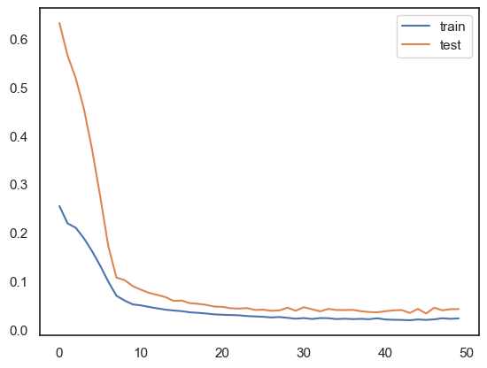
# plot history
plt.plot(history.history["loss"], label="train")
plt.plot(history.history["val_loss"], label="test")
plt.legend()
plt.show()
def predict(model, date_train, X_train, future_steps, ds):
    # Extracting dates
    dates = pd.date_range(list(date_train)[-1], periods=future, freq="1d").tolist()
    # use the last future steps from X_train
    predicted = model.predict(X_train[-future_steps:])
    predicted = np.repeat(predicted, ds.shape[1], axis=-1)
    nsamples, nx, ny = predicted.shape
    predicted = predicted.reshape((nsamples, nx * ny))

    return predicted, dates


def output_preparation(
    forecasting_dates, predictions, date_column="date", predicted_column="Volume USDT"
):
    dates = []
    for date in forecasting_dates:
        dates.append(date.date())
    predicted_df = pd.DataFrame(columns=[date_column, predicted_column])
    predicted_df[date_column] = pd.to_datetime(dates)
    predicted_df[predicted_column] = predictions
    return predicted_df


def results(
    df, lookback, future, scaler, col, X_train, y_train, df_train, date_train, model
):
    predictions, forecasting_dates = predict(model, date_train, X_train, future, df)
    results = output_preparation(forecasting_dates, predictions)
    print(results.head())
# if you need a model trained, you can use this cell
import tensorflow as tf
from tensorflow.keras.models import load_model
from tensorflow.keras.utils import get_file

model_url = "https://static-1300131294.cos.ap-shanghai.myqcloud.com/data/deep-learning/LSTM/LSTM_model.h5"
model_path = get_file("LSTM_model.h5", model_url)
LSTM_model = load_model(model_path)
Downloading data from https://static-1300131294.cos.ap-shanghai.myqcloud.com/data/deep-learning/LSTM/LSTM_model.h5
32208/32208 [==============================] - 0s 1us/step
# make a prediction
yhat = model.predict(test_X)
test_X = test_X.reshape(
    (
        test_X.shape[0],
        n_hours * n_features,
    )
)
# invert scaling for forecast
inv_yhat = concatenate((yhat, test_X[:, -4:]), axis=1)
inv_yhat = scaler.inverse_transform(inv_yhat)
inv_yhat = inv_yhat[:, 0]
# invert scaling for actual
test_y = test_y.reshape((len(test_y), 1))
inv_y = concatenate((test_y, test_X[:, -4:]), axis=1)
inv_y = scaler.inverse_transform(inv_y)
inv_y = inv_y[:, 0]
# calculate RMSE
mse = mean_squared_error(inv_y, inv_yhat)
print("Test MSE: %.3f" % mse)
rmse = sqrt(mean_squared_error(inv_y, inv_yhat))
print("Test RMSE: %.3f" % rmse)
3/3 [==============================] - 0s 2ms/step
Test MSE: 12919.827
Test RMSE: 113.665
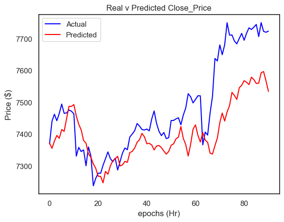
plt.title("Real v Predicted Close_Price")
plt.ylabel("Price ($)")
plt.xlabel("epochs (Hr)")

actual_values = inv_y
predicted_values = inv_yhat

# plot
plt.plot(actual_values, label="Actual", color="blue")
plt.plot(predicted_values, label="Predicted", color="red")

# set title and label
plt.title("Real v Predicted Close_Price")
plt.ylabel("Price ($)")
plt.xlabel("epochs (Hr)")

# show
plt.legend()
plt.show()
plt.show()
42.103. Acknowledgements#
Thanks to Paul Simpson for creating Bitcoin Lstm Model with Tweet Volume and Sentiment. It inspires the majority of the content in this chapter.