NumPy
Contents
5.3. NumPy#
NumPy is the fundamental package for scientific computing in Python. It is a Python library that provides a multidimensional array object, various derived objects (such as masked arrays and matrices), and an assortment of routines for fast operations on arrays, including mathematical, logical, shape manipulation, sorting, selecting, I/O, discrete Fourier transforms, basic linear algebra, basic statistical operations, random simulation and much more.
5.3.1. Basic introduction to array#
NumPy’s main object is the homogeneous multidimensional array. It is a table of elements (usually numbers), all of the same type, indexed by a tuple of non-negative integers. In NumPy dimensions are called axes.
For example, the array for the coordinates of a point in 3D space, [1, 2, 1], has one axis. That axis has 3 elements in it, so we say it has a length of 3. In the example pictured below, the array has 2 axes. The first axis has a length of 2, the second axis has a length of 3.
[[1., 0., 0.],
 [0., 1., 2.]]
[[1.0, 0.0, 0.0], [0.0, 1.0, 2.0]]
5.3.1.1. Create a basic array#
To create a NumPy array, you can use the function np.array().
All you need to do to create a simple array is pass a list to it. If you choose to, you can also specify the type of data in your list.
import numpy as np
a = np.array([1, 2, 3])
a
array([1, 2, 3])
Besides creating an array from a sequence of elements, you can easily create an array filled with 0’s:
np.zeros(2)
array([0., 0.])
Or an array filled with 1’s:
np.ones(2)
array([1., 1.])
Or even an empty array! The function empty creates an array whose initial content is random and depends on the state of the memory. The reason to use empty over zeros (or something similar) is speed - just make sure to fill every element afterwards!
np.empty(2)
array([1., 1.])
You can create an array with a range of elements:
np.arange(4)
array([0, 1, 2, 3])
And even an array that contains a range of evenly spaced intervals. To do this, you will specify the first number, last number, and the step size.
np.arange(2, 9, 2)
array([2, 4, 6, 8])
You can also use np.linspace() to create an array with values that are spaced linearly in a specified interval:
np.linspace(0, 10, num=5)
array([ 0. , 2.5, 5. , 7.5, 10. ])
While the default data type is floating point (np.float64), you can explicitly specify which data type you want using the dtype keyword.
np.ones(2, dtype=np.int64)
array([1, 1])
5.3.1.2. Adding, removing, and sorting elements#
Sorting an element is simple with np.sort(). You can specify the axis, kind, and order when you call the function.
If you start with this array:
arr = np.array([2, 1, 5, 3, 7, 4, 6, 8])
You can quickly sort the numbers in ascending order with:
np.sort(arr)
array([1, 2, 3, 4, 5, 6, 7, 8])
In addition to sort, which returns a sorted copy of an array, you can use:
argsort, which is an indirect sort along a specified axis,lexsort, which is an indirect stable sort on multiple keys,searchsorted, which will find elements in a sorted array,partition, which is a partial sort.
If you start with these arrays:
a = np.array([1, 2, 3, 4])
b = np.array([5, 6, 7, 8])
You can concatenate them with np.concatenate().
np.concatenate((a, b))
array([1, 2, 3, 4, 5, 6, 7, 8])
Or, if you start with these arrays:
x = np.array([[1, 2], [3, 4]])
y = np.array([[5, 6]])
You can concatenate them with:
np.concatenate((x, y), axis=0)
array([[1, 2],
       [3, 4],
       [5, 6]])
In order to remove elements from an array, it’s simple to use indexing to select the elements that you want to keep.
5.3.1.3. NumPy array attributes#
NumPy’s array class is called ndarray. It is also known by the alias array. Note that numpy.array is not the same as the Standard Python Library class array.array, which only handles one-dimensional arrays and offers less functionality. The more important attributes of an ndarray object are:
ndarray.ndim The number of axes (dimensions) of the array.
import numpy as np
a = np.arange(15).reshape(3, 5)
a
array([[ 0,  1,  2,  3,  4],
       [ 5,  6,  7,  8,  9],
       [10, 11, 12, 13, 14]])
a.ndim
2
ndarray.shape The dimensions of the array. This is a tuple of integers indicating the size of the array in each dimension. For a matrix with n rows and m columns,
shapewill be(n,m). The length of theshapetuple is therefore the number of axes,ndim.
a.shape
(3, 5)
ndarray.size The total number of elements of the array. This is equal to the product of the elements of
shape.
a.size
15
ndarray.dtype An object describing the type of the elements in the array. One can create or specify dtype’s using standard Python types. Additionally NumPy provides types of its own. numpy.int32, numpy.int16, and numpy.float64 are some examples.
a.dtype
dtype('int64')
a.dtype.name
'int64'
ndarray.itemsize The size in bytes of each element of the array. For example, an array of elements of type
float64hasitemsize8 (=64/8), while one of typecomplex32hasitemsize4 (=32/8). It is equivalent tondarray.dtype.itemsize.
a.itemsize
8
ndarray.data The buffer containing the actual elements of the array. Normally, we won’t need to use this attribute because we will access the elements in an array using indexing facilities.
a.data
<memory at 0x7f10d467f040>
5.3.1.4. Reshape an array#
Using arr.reshape() will give a new shape to an array without changing the data. Just remember that when you use the reshape method, the array you want to produce needs to have the same number of elements as the original array. If you start with an array with 12 elements, you’ll need to make sure that your new array also has a total of 12 elements.
If you start with this array:
a = np.arange(6)
a
array([0, 1, 2, 3, 4, 5])
You can use reshape() to reshape your array. For example, you can reshape this array to an array with three rows and two columns:
b = a.reshape(3, 2)
b
array([[0, 1],
       [2, 3],
       [4, 5]])
With np.reshape, you can specify a few optional parameters:
np.reshape(a, newshape=(1, 6), order='C')
array([[0, 1, 2, 3, 4, 5]])
a is the array to be reshaped.
newshape is the new shape you want. You can specify an integer or a tuple of integers. If you specify an integer, the result will be an array of that length. The shape should be compatible with the original shape.
order: C means to read/write the elements using C-like index order, F means to read/write the elements using Fortran-like index order, A means to read/write the elements in Fortran-like index order if a is Fortran contiguous in memory, C-like order otherwise. (This is an optional parameter and doesn’t need to be specified.)
5.3.1.5. Convert a 1D array into a 2D array(add a new axis to an array)#
You can use np.newaxis and np.expand_dims to increase the dimensions of your existing array.
Using np.newaxis will increase the dimensions of your array by one dimension when used once. This means that a 1D array will become a 2D array, a 2D array will become a 3D array, and so on.
For example, if you start with this array:
a = np.array([1, 2, 3, 4, 5, 6])
a.shape
(6,)
You can use np.newaxis to add a new axis:
a2 = a[np.newaxis, :]
a2.shape
(1, 6)
You can explicitly convert a 1D array with either a row vector or a column vector using np.newaxis. For example, you can convert a 1D array to a row vector by inserting an axis along the first dimension:
row_vector = a[np.newaxis, :]
row_vector.shape
(1, 6)
Or, for a column vector, you can insert an axis along the second dimension:
col_vector = a[:, np.newaxis]
col_vector.shape
(6, 1)
You can also expand an array by inserting a new axis at a specified position with np.expand_dims.
For example, if you start with this array:
a = np.array([1, 2, 3, 4, 5, 6])
a.shape
(6,)
You can use np.expand_dims to add an axis at index position 1 with:
b = np.expand_dims(a, axis=1)
b.shape
(6, 1)
You can add an axis at index position 0 with:
c = np.expand_dims(a, axis=0)
c.shape
(1, 6)
5.3.1.6. Indexing and slicing#
You can index and slice NumPy arrays in the same ways you can slice Python lists.
data = np.array([1, 2, 3])
data[1]
2
data[0:2]
array([1, 2])
data[1:]
array([2, 3])
data[-2:]
array([2, 3])
You may want to take a section of your array or specific array elements to use in further analysis or additional operations. To do that, you’ll need to subset, slice, and/or index your arrays.
If you want to select values from your array that fulfill certain conditions, it’s straightforward with NumPy.
For example, if you start with this array:
a = np.array([[1 , 2, 3, 4], [5, 6, 7, 8], [9, 10, 11, 12]])
You can easily print all of the values in the array that are less than 5.
a[a < 5]
array([1, 2, 3, 4])
You can also select, for example, numbers that are equal to or greater than 5, and use that condition to index an array.
five_up = (a >= 5)
a[five_up]
array([ 5, 6, 7, 8, 9, 10, 11, 12])
You can select elements that are divisible by 2:
divisible_by_2 = a[a%2==0]
divisible_by_2
array([ 2, 4, 6, 8, 10, 12])
Or you can select elements that satisfy two conditions using the & and | operators:
c = a[(a > 2) & (a < 11)]
c
array([ 3, 4, 5, 6, 7, 8, 9, 10])
You can also make use of the logical operators & and | in order to return boolean values that specify whether or not the values in an array fulfill a certain condition. This can be useful with arrays that contain names or other categorical values.
five_up = (a > 5) | (a == 5)
five_up
array([[False, False, False, False],
       [ True,  True,  True,  True],
       [ True,  True,  True,  True]])
You can also use np.nonzero() to select elements or indices from an array.
Starting with this array:
a = np.array([[1, 2, 3, 4], [5, 6, 7, 8], [9, 10, 11, 12]])
You can use np.nonzero() to print the indices of elements that are, for example, less than 5:
b = np.nonzero(a < 5)
b
(array([0, 0, 0, 0]), array([0, 1, 2, 3]))
In this example, a tuple of arrays was returned: one for each dimension. The first array represents the row indices where these values are found, and the second array represents the column indices where the values are found.
If you want to generate a list of coordinates where the elements exist, you can zip the arrays, iterate over the list of coordinates, and print them. For example:
list_of_coordinates= list(zip(b[0], b[1]))
for coord in list_of_coordinates:
    print(coord)
(0, 0)
(0, 1)
(0, 2)
(0, 3)
You can also use np.nonzero() to print the elements in an array that are less than 5 with:
a[b]
array([1, 2, 3, 4])
If the element you’re looking for doesn’t exist in the array, then the returned array of indices will be empty. For example:
not_there = np.nonzero(a == 42)
not_there
(array([], dtype=int64), array([], dtype=int64))
5.3.1.7. Create an array from existing data#
You can easily create a new array from a section of an existing array.
Let’s say you have this array:
a = np.array([1, 2, 3, 4, 5, 6, 7, 8, 9, 10])
You can create a new array from a section of your array any time by specifying where you want to slice your array.
arr1 = a[3:8]
arr1
array([4, 5, 6, 7, 8])
Here, you grabbed a section of your array from index position 3 through index position 8.
You can also stack two existing arrays, both vertically and horizontally. Let’s say you have two arrays, a1 and a2:
a1 = np.array([[1, 1],
               [2, 2]])
a2 = np.array([[3, 3],
               [4, 4]])
You can stack them vertically with vstack:
np.vstack((a1, a2))
array([[1, 1],
       [2, 2],
       [3, 3],
       [4, 4]])
Or stack them horizontally with hstack:
np.hstack((a1, a2))
array([[1, 1, 3, 3],
       [2, 2, 4, 4]])
You can split an array into several smaller arrays using hsplit. You can specify either the number of equally shaped arrays to return or the columns after which the division should occur.
Let’s say you have this array:
x = np.arange(1, 25).reshape(2, 12)
x
array([[ 1,  2,  3,  4,  5,  6,  7,  8,  9, 10, 11, 12],
       [13, 14, 15, 16, 17, 18, 19, 20, 21, 22, 23, 24]])
If you wanted to split this array into three equally shaped arrays, you would run:
np.hsplit(x, 3)
[array([[ 1,  2,  3,  4],
        [13, 14, 15, 16]]),
 array([[ 5,  6,  7,  8],
        [17, 18, 19, 20]]),
 array([[ 9, 10, 11, 12],
        [21, 22, 23, 24]])]
If you wanted to split your array after the third and fourth column, you’d run:
np.hsplit(x, (3, 4))
[array([[ 1,  2,  3],
        [13, 14, 15]]),
 array([[ 4],
        [16]]),
 array([[ 5,  6,  7,  8,  9, 10, 11, 12],
        [17, 18, 19, 20, 21, 22, 23, 24]])]
You can use the view method to create a new array object that looks at the same data as the original array (a shallow copy).
Views are an important NumPy concept! NumPy functions, as well as operations like indexing and slicing, will return views whenever possible. This saves memory and is faster (no copy of the data has to be made). However it’s important to be aware of this - modifying data in a view also modifies the original array!
Let’s say you create this array:
a = np.array([[1, 2, 3, 4], [5, 6, 7, 8], [9, 10, 11, 12]])
Now we create an array b1 by slicing a and modify the first element of b1. This will modify the corresponding element in a as well!
b1 = a[0, :]
b1
array([1, 2, 3, 4])
b1[0] = 99
b1
array([99, 2, 3, 4])
a
array([[99,  2,  3,  4],
       [ 5,  6,  7,  8],
       [ 9, 10, 11, 12]])
Using the copy method will make a complete copy of the array and its data (a deep copy). To use this on your array, you could run:
b2 = a.copy()
5.3.2. Array operations#
5.3.2.1. Basic array operations#
Once you’ve created your arrays, you can start to work with them. Let’s say, for example, that you’ve created two arrays, one called data and one called ones.
data = np.array([1, 2])
ones = np.ones(2, dtype=int)
You can add the arrays together with the plus sign.
data + ones
array([2, 3])
You can, of course, do more than just addition!
print(data - ones)
print(data * data)
print(data / data)
[0 1]
[1 4]
[1. 1.]
Basic operations are simple with NumPy. If you want to find the sum of the elements in an array, you’d use sum(). This works for 1D arrays, 2D arrays, and arrays in higher dimensions.
a = np.array([1, 2, 3, 4])
a.sum()
10
To add the rows or the columns in a 2D array, you would specify the axis.
If you start with this array:
b = np.array([[1, 1], [2, 2]])
You can sum over the axis of rows with:
b.sum(axis=0)
array([3, 3])
You can sum over the axis of columns with:
b.sum(axis=1)
array([2, 4])
5.3.2.2. Universal functions(ufunc)#
A universal function (or ufunc for short) is a function that operates on ndarrays in an element-by-element fashion, supporting array broadcasting, type casting, and several other standard features. That is, a ufunc is a “vectorized” wrapper for a function that takes a fixed number of specific inputs and produces a fixed number of specific outputs.
5.3.2.2.1. Available ufuncs#
There are currently more than 60 universal functions defined in numpy on one or more types, covering a wide variety of operations. Some of these ufuncs are called automatically on arrays when the relevant infix notation is used (e.g., add(a, b) is called internally when a + b is written and a or b is an ndarray). Nevertheless, you may still want to use the ufunc call in order to use the optional output argument(s) to place the output(s) in an object (or objects) of your choice.
Recall that each ufunc operates element-by-element. Therefore, each scalar ufunc will be described as if acting on a set of scalar inputs to return a set of scalar outputs.
Note
The ufunc still returns its output(s) even if you use the optional output argument(s).
5.3.2.2.1.1. Math operations#
Syntax |
Role |
|---|---|
|
Add arguments element-wise. |
|
Subtract arguments, element-wise. |
|
Multiply arguments element-wise. |
|
Matrix product of two arrays. |
|
Divide arguments element-wise. |
|
Logarithm of the sum of exponentiations of the inputs. |
|
Numerical negative, element-wise. |
|
Numerical positive, element-wise. |
|
First array elements raised to powers from second array, element-wise. |
|
Calculate the absolute value element-wise. |
|
Calculate the exponential of all elements in the input array. |
|
Natural logarithm, element-wise. |
|
Base-2 logarithm of x. |
5.3.2.2.1.2. Trigonometric functions#
Syntax |
Role |
|---|---|
|
Trigonometric sine, element-wise. |
|
Cosine element-wise. |
|
Compute tangent element-wise. |
|
Inverse sine, element-wise. |
|
Trigonometric inverse cosine, element-wise. |
|
Trigonometric inverse tangent, element-wise. |
5.3.2.2.1.3. Bit-twiddling functions#
Syntax |
Role |
|---|---|
|
Compute the bit-wise AND of two arrays element-wise. |
|
Compute the bit-wise OR of two arrays element-wise. |
|
Compute the bit-wise XOR of two arrays element-wise. |
|
Compute bit-wise inversion, or bit-wise NOT, element-wise. |
5.3.2.2.1.4. Comparison functions#
Syntax |
Role |
|---|---|
|
Return the truth value of (x1 > x2) element-wise. |
|
Return the truth value of (x1 >= x2) element-wise. |
|
Return the truth value of (x1 < x2) element-wise. |
|
Return the truth value of (x1 <= x2) element-wise. |
|
Return (x1 != x2) element-wise. |
|
Return (x1 == x2) element-wise. |
Warning
Do not use the Python keywords and and or to combine logical array expressions. These keywords will test the truth value of the entire array (not element-by-element as you might expect). Use the bitwise operators & and | instead.
Syntax |
Role |
|---|---|
|
Compute the truth value of x1 AND x2 element-wise. |
|
Compute the truth value of x1 OR x2 element-wise. |
|
Compute the truth value of x1 XOR x2, element-wise. |
|
Compute the truth value of NOT x element-wise. |
Warning
The bit-wise operators & and | are the proper way to perform element-by-element array comparisons. Be sure you understand the operator precedence: (a > 2) & (a < 5) is the proper syntax because a > 2 & a < 5 will result in an error due to the fact that 2 & a is evaluated first.
5.3.2.3. Computation on arrays: broadcasting#
The term broadcasting describes how NumPy treats arrays with different shapes during arithmetic operations. Subject to certain constraints, the smaller array is “broadcast” across the larger array so that they have compatible shapes. Broadcasting provides a means of vectorizing array operations so that looping occurs in C instead of Python. It does this without making needless copies of data and usually leads to efficient algorithm implementations. There are, however, cases where broadcasting is a bad idea because it leads to inefficient use of memory that slows computation.
NumPy operations are usually done on pairs of arrays on an element-by-element basis. In the simplest case, the two arrays must have exactly the same shape, as in the following example:
a = np.array([1.0, 2.0, 3.0])
b = np.array([2.0, 2.0, 2.0])
a * b
array([2., 4., 6.])
NumPy’s broadcasting rule relaxes this constraint when the arrays’ shapes meet certain constraints. The simplest broadcasting example occurs when an array and a scalar value are combined in an operation:
a = np.array([1.0, 2.0, 3.0])
b = 2.0
a * b
array([2., 4., 6.])
The result is equivalent to the previous example where b was an array. NumPy is smart enough to use the original scalar value without actually making copies so that broadcasting operations are as memory and computationally efficient as possible.
5.3.2.3.1. General Broadcasting Rules#
When operating on two arrays, NumPy compares their shapes element-wise. It starts with the trailing (i.e. rightmost) dimension and works its way left. Two dimensions are compatible when
they are equal, or
one of them is 1.
If these conditions are not met, a ValueError: operands could not be broadcast together exception is thrown, indicating that the arrays have incompatible shapes.
Input arrays do not need to have the same number of dimensions. The resulting array will have the same number of dimensions as the input array with the greatest number of dimensions, where the size of each dimension is the largest size of the corresponding dimension among the input arrays. Note that missing dimensions are assumed to have size one.
For example, if you have a 256x256x3 array of RGB values, and you want to scale each color in the image by a different value, you can multiply the image by a one-dimensional array with 3 values. Lining up the sizes of the trailing axes of these arrays according to the broadcast rules, shows that they are compatible:
Image  (3d array): 256 x 256 x 3
Scale  (1d array):             3
Result (3d array): 256 x 256 x 3
When either of the dimensions compared is one, the other is used. In other words, dimensions with size 1 are stretched or “copied” to match the other.
In the following example, both the A and B arrays have axes with length one that are expanded to a larger size during the broadcast operation:
A      (4d array):  8 x 1 x 6 x 1
B      (3d array):      7 x 1 x 5
Result (4d array):  8 x 7 x 6 x 5
5.3.2.4. Aggregations: min, max and everything in between#
NumPy also performs aggregation functions. In addition to min, max, and sum, you can easily run mean to get the average, prod to get the result of multiplying the elements together, std to get the standard deviation, and more.
data.max()
2
data.min()
1
data.sum()
3
Let’s start with this array, called “a”.
a = np.array([[0.45053314, 0.17296777, 0.34376245, 0.5510652],
              [0.54627315, 0.05093587, 0.40067661, 0.55645993],
              [0.12697628, 0.82485143, 0.26590556, 0.56917101]])
It’s very common to want to aggregate along a row or column. By default, every NumPy aggregation function will return the aggregate of the entire array. To find the sum or the minimum of the elements in your array, run:
a.sum()
4.8595784
Or:
a.min()
0.05093587
You can specify on which axis you want the aggregation function to be computed. For example, you can find the minimum value within each column by specifying axis=0.
a.min(axis=0)
array([0.12697628, 0.05093587, 0.26590556, 0.5510652 ])
The four values listed above correspond to the number of columns in your array. With a four-column array, you will get four values as your result.
5.3.3. Indexing on ndarrays#
ndarrays can be indexed using the standard Python x[obj] syntax, where x is the array and obj the selection. There are different kinds of indexing available depending on obj: basic indexing, advanced indexing and field access.
Note
In Python, x[(exp1, exp2, ..., expN)] is equivalent to x[exp1, exp2, ..., expN]; the latter is just syntactic sugar for the former.
5.3.3.1. Basic indexing#
5.3.3.1.1. Single element indexing#
Single element indexing works exactly like that for other standard Python sequences. It is 0-based, and accepts negative indices for indexing from the end of the array.
x = np.arange(10)
x[2]
2
x[-2]
8
It is not necessary to separate each dimension’s index into its own set of square brackets.
x.shape = (2, 5) # now x is 2-dimensional
x[1, 3]
8
x[1, -1]
9
Note that If one indexes a multidimensional array with fewer indices than dimensions, one gets a subdimensional array. For example:
x[0]
array([0, 1, 2, 3, 4])
That is, each index specified selects the array corresponding to the rest of the dimensions selected. In the above example, choosing 0 means that the remaining dimension of length 5 is being left unspecified, and that what is returned is an array of that dimensionality and size. It must be noted that the returned array is a view, i.e., it is not a copy of the original, but points to the same values in memory as does the original array. In this case, the 1-D array at the first position (0) is returned. So using a single index on the returned array, results in a single element being returned. That is:
x[0][2]
2
So note that x[0, 2] == x[0][2] though the second case is more inefficient as a new temporary array is created after the first index that is subsequently indexed by 2.
Note
NumPy uses C-order indexing. That means that the last index usually represents the most rapidly changing memory location, unlike Fortran or IDL, where the first index represents the most rapidly changing location in memory. This difference represents a great potential for confusion.
5.3.3.1.2. Slicing and striding#
Basic slicing extends Python’s basic concept of slicing to N dimensions. Basic slicing occurs when obj is a slice object (constructed by start:stop:step notation inside of brackets), an integer, or a tuple of slice objects and integers. Ellipsis and newaxis objects can be interspersed with these as well.
The simplest case of indexing with N integers returns an array scalar representing the corresponding item. As in Python, all indices are zero-based: for the i-th index , the valid range is \(0 \leq n_i \leq d_i\) where \(d_i\) is the i-th element of the shape of the array. Negative indices are interpreted as counting from the end of the array (i.e., if , it \(n_i < 0\), it means \(n_i + d_i\)).
All arrays generated by basic slicing are always views of the original array.
Note
NumPy slicing creates a view instead of a copy as in the case of built-in Python sequences such as string, tuple and list. Care must be taken when extracting a small portion from a large array which becomes useless after the extraction, because the small portion extracted contains a reference to the large original array whose memory will not be released until all arrays derived from it are garbage-collected. In such cases an explicit copy() is recommended.
The basic slice syntax is
i:j:kwhere i is the starting index, j is the stopping index, and k is the step (\(k /neq 0\)). This selects the m elements (in the corresponding dimension) with index values i, i + k, …,i + (m - 1) k where \(m = q + (r /neq 0)\) and q and r are the quotient and remainder obtained by dividing j - i by k: j - i = q k + r, so that i + (m - 1) k < j. For example:
x = np.array([0, 1, 2, 3, 4, 5, 6, 7, 8, 9])
x[1:7:2]
array([1, 3, 5])
Negative i and j are interpreted as n + i and n + j where n is the number of elements in the corresponding dimension. Negative k makes stepping go towards smaller indices. From the above example:
x[-2:10]
array([8, 9])
x[-3:3:-1]
array([7, 6, 5, 4])
Assume n is the number of elements in the dimension being sliced. Then, if i is not given it defaults to 0 for k > 0 and n - 1 for k < 0. If j is not given it defaults to n for k > 0 and -n-1 for k < 0. If k is not given it defaults to 1. Note that
::is the same as : and means select all indices along this axis. From the above example:
x[5:]
array([5, 6, 7, 8, 9])
If the number of objects in the selection tuple is less than N, then
:is assumed for any subsequent dimensions. For example:
x = np.array([[[1],[2],[3]], [[4],[5],[6]]])
x.shape
(2, 3, 1)
x[1:2]
array([[[4],
        [5],
        [6]]])
An integer, i, returns the same values as
i:i+1except the dimensionality of the returned object is reduced by 1. In particular, a selection tuple with the p-th element an integer (and all other entries :) returns the corresponding sub-array with dimension N - 1. If N = 1 then the returned object is an array scalar.If the selection tuple has all entries : except the p-th entry which is a slice object
i:j:k, then the returned array has dimension N formed by concatenating the sub-arrays returned by integer indexing of elements i, i+k, …, i + (m - 1) k < j,Basic slicing with more than one non-
:entry in the slicing tuple, acts like repeated application of slicing using a single non-:entry, where the non-:entries are successively taken (with all other non-:entries replaced by:). Thus,x[ind1, ..., ind2,:]acts likex[ind1][..., ind2, :]under basic slicing.
WARNING: The The above is not true for advanced indexing.
You may use slicing to set values in the array, but (unlike lists) you can never grow the array. The size of the value to be set in
x[obj] = valuemust be (broadcastable) to the same shape asx[obj].A slicing tuple can always be constructed as obj and used in the
x[obj]notation. Slice objects can be used in the construction in place of the[start:stop:step]notation. For example,x[1:10:5, ::-1]can also be implemented asobj = (slice(1, 10, 5), slice(None, None, -1));x[obj]. This can be useful for constructing generic code that works on arrays of arbitrary dimensions.
5.3.3.1.3. Dimensional indexing tools#
There are some tools to facilitate the easy matching of array shapes with expressions and in assignments.
Ellipsis expands to the number of : objects needed for the selection tuple to index all dimensions. In most cases, this means that the length of the expanded selection tuple is x.ndim. There may only be a single ellipsis present. From the above example:
x[..., 0]
array([[1, 2, 3],
       [4, 5, 6]])
This is equivalent to:
x[:, :, 0]
array([[1, 2, 3],
       [4, 5, 6]])
Each newaxis object in the selection tuple serves to expand the dimensions of the resulting selection by one unit-length dimension. The added dimension is the position of the newaxis object in the selection tuple. newaxis is an alias for None, and None can be used in place of this with the same result. From the above example:
x[:, np.newaxis, :, :].shape
(2, 1, 3, 1)
x[:, None, :, :].shape
(2, 1, 3, 1)
This can be handy to combine two arrays in a way that otherwise would require explicit reshaping operations. For example:
x = np.arange(5)
x[:, np.newaxis] + x[np.newaxis, :]
array([[0, 1, 2, 3, 4],
       [1, 2, 3, 4, 5],
       [2, 3, 4, 5, 6],
       [3, 4, 5, 6, 7],
       [4, 5, 6, 7, 8]])
5.3.3.2. Advanced indexing#
Advanced indexing is triggered when the selection object, obj, is a non-tuple sequence object, an ndarray (of data type integer or bool), or a tuple with at least one sequence object or ndarray (of data type integer or bool). There are two types of advanced indexing: integer and Boolean.
Advanced indexing always returns a copy of the data (contrast with basic slicing that returns a view).
WARNING: The definition of advanced indexing means that x[(1, 2, 3),] is fundamentally different than x[(1, 2, 3)]. The latter is equivalent to x[1, 2, 3] which will trigger basic selection while the former will trigger advanced indexing. Be sure to understand why this occurs.
Also recognize that x[[1, 2, 3]] will trigger advanced indexing, whereas due to the deprecated Numeric compatibility mentioned above, x[[1, 2, slice(None)]] will trigger basic slicing.
5.3.3.2.1. Integer array indexing#
Integer array indexing allows selection of arbitrary items in the array based on their N-dimensional index. Each integer array represents a number of indices into that dimension.
Negative values are permitted in the index arrays and work as they do with single indices or slices:
x = np.arange(10, 1, -1)
x
array([10, 9, 8, 7, 6, 5, 4, 3, 2])
x[np.array([3, 3, 1, 8])]
array([7, 7, 9, 2])
x[np.array([3, 3, -3, 8])]
array([7, 7, 4, 2])
If the index values are out of bounds then an IndexError is thrown:
x = np.array([[1, 2], [3, 4], [5, 6]])
x[np.array([1, -1])]
array([[3, 4],
       [5, 6]])
x[np.array([3, 4])]
Traceback (most recent call last):
  ...
IndexError: index 3 is out of bounds for axis 0 with size 3
When the index consists of as many integer arrays as dimensions of the array being indexed, the indexing is straightforward, but different from slicing.
Advanced indices always are broadcast and iterated as one:
result[i_1, ..., i_M] == x[ind_1[i_1, ..., i_M], ind_2[i_1, ..., i_M],
                           ..., ind_N[i_1, ..., i_M]]
Note that the resulting shape is identical to the (broadcast) indexing array shapes ind_1, ..., ind_N. If the indices cannot be broadcast to the same shape, an exception IndexError: shape mismatch: indexing arrays could not be broadcast together with shapes... is raised.
Indexing with multidimensional index arrays tend to be more unusual uses, but they are permitted, and they are useful for some problems. We’ll start with the simplest multidimensional case:
y = np.arange(35).reshape(5, 7)
y
array([[ 0,  1,  2,  3,  4,  5,  6],
       [ 7,  8,  9, 10, 11, 12, 13],
       [14, 15, 16, 17, 18, 19, 20],
       [21, 22, 23, 24, 25, 26, 27],
       [28, 29, 30, 31, 32, 33, 34]])
y[np.array([0, 2, 4]), np.array([0, 1, 2])]
array([ 0, 15, 30])
In this case, if the index arrays have a matching shape, and there is an index array for each dimension of the array being indexed, the resultant array has the same shape as the index arrays, and the values correspond to the index set for each position in the index arrays. In this example, the first index value is 0 for both index arrays, and thus the first value of the resultant array is y[0, 0]. The next value is y[2, 1], and the last is y[4, 2].
If the index arrays do not have the same shape, there is an attempt to broadcast them to the same shape. If they cannot be broadcast to the same shape, an exception is raised:
y[np.array([0, 2, 4]), np.array([0, 1])]
Traceback (most recent call last):
  ...
IndexError: shape mismatch: indexing arrays could not be broadcast together with shapes (3,) (2,)
The broadcasting mechanism permits index arrays to be combined with scalars for other indices. The effect is that the scalar value is used for all the corresponding values of the index arrays:
y[np.array([0, 2, 4]), 1]
array([ 1, 15, 29])
Jumping to the next level of complexity, it is possible to only partially index an array with index arrays. It takes a bit of thought to understand what happens in such cases. For example if we just use one index array with y:
y[np.array([0, 2, 4])]
array([[ 0,  1,  2,  3,  4,  5,  6],
       [14, 15, 16, 17, 18, 19, 20],
       [28, 29, 30, 31, 32, 33, 34]])
It results in the construction of a new array where each value of the index array selects one row from the array being indexed and the resultant array has the resulting shape (number of index elements, size of row).
In general, the shape of the resultant array will be the concatenation of the shape of the index array (or the shape that all the index arrays were broadcast to) with the shape of any unused dimensions (those not indexed) in the array being indexed.
5.3.3.2.1.1. Example 1#
From each row, a specific element should be selected. The row index is just [0, 1, 2] and the column index specifies the element to choose for the corresponding row, here [0, 1, 0]. Using both together the task can be solved using advanced indexing:
x = np.array([[1, 2], [3, 4], [5, 6]])
x[[0, 1, 2], [0, 1, 0]]
array([1, 4, 5])
To achieve a behaviour similar to the basic slicing above, broadcasting can be used. The function ix_ can help with this broadcasting. This is best understood with an example.
5.3.3.2.1.2. Example 2#
From a \(4x3\) array the corner elements should be selected using advanced indexing. Thus all elements for which the column is one of [0, 2] and the row is one of [0, 3] need to be selected. To use advanced indexing one needs to select all elements explicitly. Using the method explained previously one could write:
x = np.array([[ 0,  1,  2],
              [ 3,  4,  5],
              [ 6,  7,  8],
              [ 9, 10, 11]])
rows = np.array([[0, 0],
                 [3, 3]], dtype=np.intp)
columns = np.array([[0, 2],
                    [0, 2]], dtype=np.intp)
x[rows, columns]
array([[ 0,  2],
       [ 9, 11]])
However, since the indexing arrays above just repeat themselves, broadcasting can be used (compare operations such as rows[:, np.newaxis] + columns) to simplify this:
rows = np.array([0, 3], dtype=np.intp)
columns = np.array([0, 2], dtype=np.intp)
rows[:, np.newaxis]
array([[0],
       [3]])
x[rows[:, np.newaxis], columns]
array([[ 0,  2],
       [ 9, 11]])
This broadcasting can also be achieved using the function ix_:
x[np.ix_(rows, columns)]
array([[ 0,  2],
       [ 9, 11]])
Note that without the np.ix_ call, only the diagonal elements would be selected:
x[rows, columns]
array([ 0, 11])
This difference is the most important thing to remember about indexing with multiple advanced indices.
5.3.3.2.1.3. Example 3#
A real-life example of where advanced indexing may be useful is for a color lookup table where we want to map the values of an image into RGB triples for display. The lookup table could have a shape (nlookup, 3). Indexing such an array with an image with shape (ny, nx) with dtype=np.uint8 (or any integer type so long as values are with the bounds of the lookup table) will result in an array of shape (ny, nx, 3) where a triple of RGB values is associated with each pixel location.
5.3.3.2.2. Boolean array indexing#
This advanced indexing occurs when obj is an array object of Boolean type, such as may be returned from comparison operators. A single boolean index array is practically identical to x[obj.nonzero()] where, as described above, obj.nonzero() returns a tuple (of length obj.ndim) of integer index arrays showing the True elements of obj. However, it is faster when obj.shape == x.shape.
If obj.ndim == x.ndim, x[obj] returns a 1-dimensional array filled with the elements of x corresponding to the True values of obj. The search order will be row-major, C-style. If obj has True values at entries that are outside of the bounds of x, then an index error will be raised. If obj is smaller than x it is identical to filling it with False.
A common use case for this is filtering for desired element values. For example, one may wish to select all entries from an array which are not NaN:
x = np.array([[1., 2.], [np.nan, 3.], [np.nan, np.nan]])
x[~np.isnan(x)]
array([1., 2., 3.])
Or wish to add a constant to all negative elements:
x = np.array([1., -1., -2., 3])
x[x < 0] += 20
x
array([ 1., 19., 18., 3.])
In general if an index includes a Boolean array, the result will be identical to inserting obj.nonzero() into the same position and using the integer array indexing mechanism described above. x[ind_1, boolean_array, ind_2] is equivalent to x[(ind_1,) + boolean_array.nonzero() + (ind_2,)].
If there is only one Boolean array and no integer indexing array present, this is straightforward. Care must only be taken to make sure that the boolean index has exactly as many dimensions as it is supposed to work with.
In general, when the boolean array has fewer dimensions than the array being indexed, this is equivalent to x[b, ...], which means x is indexed by b followed by as many : as are needed to fill out the rank of x. Thus the shape of the result is one dimension containing the number of True elements of the boolean array, followed by the remaining dimensions of the array being indexed:
x = np.arange(35).reshape(5, 7)
b = x > 20
b[:, 5]
array([False, False, False, True, True])
x[b[:, 5]]
array([[21, 22, 23, 24, 25, 26, 27],
       [28, 29, 30, 31, 32, 33, 34]])
Here the 4th and 5th rows are selected from the indexed array and combined to make a 2-D array.
5.3.3.2.2.1. Example 1#
From an array, select all rows which sum up to less or equal two:
x = np.array([[0, 1], [1, 1], [2, 2]])
rowsum = x.sum(-1)
x[rowsum <= 2, :]
array([[0, 1],
       [1, 1]])
Combining multiple Boolean indexing arrays or a Boolean with an integer indexing array can best be understood with the obj.nonzero() analogy. The function ix_ also supports boolean arrays and will work without any surprises.
5.3.3.2.2.2. Example 2#
Use boolean indexing to select all rows adding up to an even number. At the same time columns 0 and 2 should be selected with an advanced integer index. Using the ix_ function this can be done with:
x = np.array([[ 0,  1,  2],
              [ 3,  4,  5],
              [ 6,  7,  8],
              [ 9, 10, 11]])
rows = (x.sum(-1) % 2) == 0
rows
array([False, True, False, True])
columns = [0, 2]
x[np.ix_(rows, columns)]
array([[ 3,  5],
       [ 9, 11]])
Without the np.ix_ call, only the diagonal elements would be selected.
Or without np.ix_ (compare the integer array examples):
rows = rows.nonzero()[0]
x[rows[:, np.newaxis], columns]
array([[ 3,  5],
       [ 9, 11]])
5.3.3.2.2.3. Example 3#
Use a 2-D boolean array of shape (2, 3) with four True elements to select rows from a 3-D array of shape (2, 3, 5) results in a 2-D result of shape (4, 5):
x = np.arange(30).reshape(2, 3, 5)
x
array([[[ 0,  1,  2,  3,  4],
        [ 5,  6,  7,  8,  9],
        [10, 11, 12, 13, 14]],

       [[15, 16, 17, 18, 19],
        [20, 21, 22, 23, 24],
        [25, 26, 27, 28, 29]]])
b = np.array([[True, True, False], [False, True, True]])
x[b]
array([[ 0,  1,  2,  3,  4],
       [ 5,  6,  7,  8,  9],
       [20, 21, 22, 23, 24],
       [25, 26, 27, 28, 29]])
5.3.3.2.3. Combining advanced and basic indexing#
When there is at least one slice (:), ellipsis (...) or newaxis in the index (or the array has more dimensions than there are advanced indices), then the behaviour can be more complicated. It is like concatenating the indexing result for each advanced index element.
In the simplest case, there is only a single advanced index combined with a slice. For example:
y = np.arange(35).reshape(5,7)
y[np.array([0, 2, 4]), 1:3]
array([[ 1,  2],
       [15, 16],
       [29, 30]])
In effect, the slice and index array operation are independent. The slice operation extracts columns with index 1 and 2, (i.e. the 2nd and 3rd columns), followed by the index array operation which extracts rows with index 0, 2 and 4 (i.e the first, third and fifth rows). This is equivalent to:
y[:, 1:3][np.array([0, 2, 4]), :]
array([[ 1,  2],
       [15, 16],
       [29, 30]])
A single advanced index can, for example, replace a slice and the result array will be the same. However, it is a copy and may have a different memory layout. A slice is preferable when it is possible. For example:
x = np.array([[ 0,  1,  2],
              [ 3,  4,  5],
              [ 6,  7,  8],
              [ 9, 10, 11]])
x[1:2, 1:3]
array([[4, 5]])
x[1:2, [1, 2]]
array([[4, 5]])
The easiest way to understand a combination of multiple advanced indices may be to think in terms of the resulting shape. There are two parts to the indexing operation, the subspace defined by the basic indexing (excluding integers) and the subspace from the advanced indexing part. Two cases of index combination need to be distinguished:
The advanced indices are separated by a slice,
Ellipsisornewaxis. For examplex[arr1, :, arr2].The advanced indices are all next to each other. For example
x[..., arr1, arr2, :]but notx[arr1, :, 1]since1is an advanced index in this regard.
In the first case, the dimensions resulting from the advanced indexing operation come first in the result array, and the subspace dimensions after that. In the second case, the dimensions from the advanced indexing operations are inserted into the result array at the same spot as they were in the initial array (the latter logic is what makes simple advanced indexing behave just like slicing).
5.3.3.2.3.1. Example 1#
Suppose x.shape is (10, 20, 30) and ind is a (2, 3, 4)-shaped indexing intp array, then result = x[..., ind, :] has shape (10, 2, 3, 4, 30) because the (20,)-shaped subspace has been replaced with a (2, 3, 4)-shaped broadcasted indexing subspace. If we let i, j, k loop over the (2, 3, 4)-shaped subspace then result[..., i, j, k, :] = x[..., ind[i, j, k], :]. This example produces the same result as x.take(ind, axis=-2).
5.3.3.2.3.2. Example 2#
Let x.shape be (10, 20, 30, 40, 50) and suppose ind_1 and ind_2 can be broadcast to the shape (2, 3, 4). Then x[:, ind_1, ind_2] has shape (10, 2, 3, 4, 40, 50) because the (20, 30)-shaped subspace from X has been replaced with the (2, 3, 4) subspace from the indices. However, x[:, ind_1, :, ind_2] has shape (2, 3, 4, 10, 30, 50) because there is no unambiguous place to drop in the indexing subspace, thus it is tacked-on to the beginning. It is always possible to use .transpose() to move the subspace anywhere desired. Note that this example cannot be replicated using take.
5.3.3.2.3.3. Example 3#
Slicing can be combined with broadcasted boolean indices:
x = np.arange(35).reshape(5, 7)
b = x > 20
b
array([[False, False, False, False, False, False, False],
       [False, False, False, False, False, False, False],
       [False, False, False, False, False, False, False],
       [ True,  True,  True,  True,  True,  True,  True],
       [ True,  True,  True,  True,  True,  True,  True]])
x[b[:, 5], 1:3]
array([[22, 23],
       [29, 30]])
5.3.3.3. Field access#
If the ndarray object is a structured array the fields of the array can be accessed by indexing the array with strings, dictionary-like.
Indexing x['field-name'] returns a new view to the array, which is of the same shape as x (except when the field is a sub-array) but of data type x.dtype['field-name'] and contains only the part of the data in the specified field. Also, record array scalars can be “indexed” this way.
Indexing into a structured array can also be done with a list of field names, e.g. x[['field-name1', 'field-name2']]. As of NumPy 1.16, this returns a view containing only those fields. In older versions of NumPy, it returned a copy. See the user guide section on Structured arrays for more information on multifield indexing.
If the accessed field is a sub-array, the dimensions of the sub-array are appended to the shape of the result. For example:
x = np.zeros((2, 2), dtype=[('a', np.int32), ('b', np.float64, (3, 3))])
x['a'].shape
(2, 2)
x['a'].dtype
dtype('int32')
x['b'].shape
(2, 2, 3, 3)
x['b'].dtype
dtype('float64')
5.3.3.4. Flat Iterator indexing#
x.flat returns an iterator that will iterate over the entire array (in C-contiguous style with the last index varying the fastest). This iterator object can also be indexed using basic slicing or advanced indexing as long as the selection object is not a tuple. This should be clear from the fact thatx.flat is a 1-dimensional view. It can be used for integer indexing with 1-dimensional C-style-flat indices. The shape of any returned array is therefore the shape of the integer indexing object.
5.3.3.5. Assigning values to indexed arrays#
As mentioned, one can select a subset of an array to assign to using a single index, slices, and index and mask arrays. The value being assigned to the indexed array must be shape consistent (the same shape or broadcastable to the shape the index produces). For example, it is permitted to assign a constant to a slice:
x = np.arange(10)
x[2:7] = 1
Or an array of the right size:
x[2:7] = np.arange(5)
Note that assignments may result in changes if assigning higher types to lower types (like floats to ints) or even exceptions (assigning complex to floats or ints):
x[1] = 1.2
x[1]
1
x[1] = 1.2j
Traceback (most recent call last):
  ...
TypeError: can't convert complex to int
Unlike some of the references (such as array and mask indices) assignments are always made to the original data in the array (indeed, nothing else would make sense!). Note though, that some actions may not work as one may naively expect. This particular example is often surprising to people:
x = np.arange(0, 50, 10)
x
array([ 0, 10, 20, 30, 40])
x[np.array([1, 1, 3, 1])] += 1
x
array([ 0, 11, 20, 31, 40])
Where people expect that the 1st location will be incremented by 3. In fact, it will only be incremented by 1. The reason is that a new array is extracted from the original (as a temporary) containing the values at 1, 1, 3, 1, then the value 1 is added to the temporary, and then the temporary is assigned back to the original array. Thus the value of the array at x[1] + 1 is assigned to x[1] three times, rather than being incremented 3 times.
5.3.3.6. Dealing with variable numbers of indices within programs#
The indexing syntax is very powerful but limiting when dealing with a variable number of indices. For example, if you want to write a function that can handle arguments with various numbers of dimensions without having to write special case code for each number of possible dimensions, how can that be done? If one supplies to the index a tuple, the tuple will be interpreted as a list of indices. For example:
z = np.arange(81).reshape(3, 3, 3, 3)
indices = (1, 1, 1, 1)
z[indices]
40
So one can use code to construct tuples of any number of indices and then use these within an index.
Slices can be specified within programs by using the slice() function in Python. For example:
indices = (1, 1, 1, slice(0, 2))  # same as [1, 1, 1, 0:2]
z[indices]
array([39, 40])
Likewise, ellipsis can be specified by code by using the Ellipsis object:
indices = (1, Ellipsis, 1)  # same as [1, ..., 1]
z[indices]
array([[28, 31, 34],
       [37, 40, 43],
       [46, 49, 52]])
For this reason, it is possible to use the output from the np.nonzero() function directly as an index since it always returns a tuple of index arrays.
Because of the special treatment of tuples, they are not automatically converted to an array as a list would be. As an example:
z[[1, 1, 1, 1]] # produces a large array
array([[[[27, 28, 29],
         [30, 31, 32],
         [33, 34, 35]],

        [[36, 37, 38],
         [39, 40, 41],
         [42, 43, 44]],

        [[45, 46, 47],
         [48, 49, 50],
         [51, 52, 53]]],


       [[[27, 28, 29],
         [30, 31, 32],
         [33, 34, 35]],

        [[36, 37, 38],
         [39, 40, 41],
         [42, 43, 44]],

        [[45, 46, 47],
         [48, 49, 50],
         [51, 52, 53]]],


       [[[27, 28, 29],
         [30, 31, 32],
         [33, 34, 35]],

        [[36, 37, 38],
         [39, 40, 41],
         [42, 43, 44]],

        [[45, 46, 47],
         [48, 49, 50],
         [51, 52, 53]]],


       [[[27, 28, 29],
         [30, 31, 32],
         [33, 34, 35]],

        [[36, 37, 38],
         [39, 40, 41],
         [42, 43, 44]],

        [[45, 46, 47],
         [48, 49, 50],
         [51, 52, 53]]]])
z[(1, 1, 1, 1)] # returns a single value
40
5.3.4. Structured arrays#
5.3.4.1. Introduction#
Structured arrays are ndarrays whose datatype is a composition of simpler datatypes organized as a sequence of named fields. For example,
x = np.array([('Rex', 9, 81.0), ('Fido', 3, 27.0)],
             dtype=[('name', 'U10'), ('age', 'i4'), ('weight', 'f4')])
x
array([('Rex', 9, 81.), ('Fido', 3, 27.)],
      dtype=[('name', '<U10'), ('age', '<i4'), ('weight', '<f4')])
Here x is a one-dimensional array of length two whose datatype is a structure with three fields: 1. A string of length 10 or less named 'name', 2. a 32-bit integer named 'age', and 3. a 32-bit float named 'weight'.
If you index x at position 1 you get a structure:
x[1]
('Fido', 3, 27.)
You can access and modify individual fields of a structured array by indexing with the field name:
x['age']
array([9, 3], dtype=int32)
x['age']
array([9, 3], dtype=int32)
x
array([('Rex', 9, 81.), ('Fido', 3, 27.)],
      dtype=[('name', '<U10'), ('age', '<i4'), ('weight', '<f4')])
Structured datatypes are designed to be able to mimic ‘structs’ in the C language, and share a similar memory layout. They are meant for interfacing with C code and for low-level manipulation of structured buffers, for example for interpreting binary blobs. For these purposes they support specialized features such as subarrays, nested datatypes, and unions, and allow control over the memory layout of the structure.
Users looking to manipulate tabular data, such as stored in csv files, may find other pydata projects more suitable, such as xarray, pandas, or DataArray. These provide a high-level interface for tabular data analysis and are better optimized for that use. For instance, the C-struct-like memory layout of structured arrays in numpy can lead to poor cache behavior in comparison.
5.3.4.2. Structured datatypes#
A structured datatype can be thought of as a sequence of bytes of a certain length (the structure’s itemsize) which is interpreted as a collection of fields. Each field has a name, a datatype, and a byte offset within the structure. The datatype of a field may be any numpy datatype including other structured datatypes, and it may also be a subarray data type which behaves like an ndarray of a specified shape. The offsets of the fields are arbitrary, and fields may even overlap. These offsets are usually determined automatically by numpy, but can also be specified.
5.3.4.2.1. Structured datatype creation#
Structured datatypes may be created using the function numpy.dtype. There are 4 alternative forms of specification which vary in flexibility and conciseness. In summary they are:
A list of tuples, one tuple per field
Each tuple has the form (fieldname, datatype, shape) where shape is optional. fieldname is a string (or tuple if titles are used, see Field Titles below), datatype may be any object convertible to a datatype, and shape is a tuple of integers specifying subarray shape.
np.dtype([('x', 'f4'), ('y', np.float32), ('z', 'f4', (2, 2))])
dtype([('x', '<f4'), ('y', '<f4'), ('z', '<f4', (2, 2))])
If fieldname is the empty string '', the field will be given a default name of the form f#, where # is the integer index of the field, counting from 0 from the left:
np.dtype([('x', 'f4'), ('', 'i4'), ('z', 'i8')])
dtype([('x', '<f4'), ('f1', '<i4'), ('z', '<i8')])
The byte offsets of the fields within the structure and the total structure itemsize are determined automatically.
A string of comma-separated dtype specifications
In this shorthand notation any of the string dtype specifications may be used in a string and separated by commas. The itemsize and byte offsets of the fields are determined automatically, and the field names are given the default names f0, f1, etc.
np.dtype('i8, f4, S3')
dtype([('f0', '<i8'), ('f1', '<f4'), ('f2', 'S3')])
np.dtype('3int8, float32, (2, 3)float64')
dtype([('f0', 'i1', (3,)), ('f1', '<f4'), ('f2', '<f8', (2, 3))])
A dictionary of field parameter arrays
This is the most flexible form of specification since it allows control over the byte-offsets of the fields and the itemsize of the structure.
The dictionary has two required keys, ‘names’ and ‘formats’, and four optional keys, 'offsets', 'itemsize', 'aligned' and ‘titles’. The values for ‘names’ and ‘formats’ should respectively be a list of field names and a list of dtype specifications, of the same length. The optional 'offsets' value should be a list of integer byte-offsets, one for each field within the structure. If 'offsets' is not given the offsets are determined automatically. The optional 'itemsize' value should be an integer describing the total size in bytes of the dtype, which must be large enough to contain all the fields.
np.dtype({'names': ['col1', 'col2'], 'formats': ['i4', 'f4']})
dtype([('col1', '<i4'), ('col2', '<f4')])
np.dtype({'names': ['col1', 'col2'],
    'formats': ['i4', 'f4'],
    'offsets': [0, 4],
    'itemsize': 12})
dtype({'names': ['col1', 'col2'], 'formats': ['<i4', '<f4'], 'offsets': [0, 4], 'itemsize': 12})
Offsets may be chosen such that the fields overlap, though this will mean that assigning to one field may clobber any overlapping field’s data. As an exception, fields of numpy.object_ type cannot overlap with other fields, because of the risk of clobbering the internal object pointer and then dereferencing it.
The optional 'aligned' value can be set to True to make the automatic offset computation use aligned offsets, as if the ‘align’ keyword argument of numpy.dtype had been set to True.
A dictionary of field names
The keys of the dictionary are the field names and the values are tuples specifying type and offset:
np.dtype({'col1': ('i1', 0), 'col2': ('f4', 1)})
dtype([('col1', 'i1'), ('col2', '<f4')])
5.3.4.2.2. Manipulating and Displaying Structured Datatypes#
The list of field names of a structured datatype can be found in the names attribute of the dtype object:
d = np.dtype([('x', 'i8'), ('y', 'f4')])
d.names
('x', 'y')
The field names may be modified by assigning to the names attribute using a sequence of strings of the same length.
The dtype object also has a dictionary-like attribute, fields, whose keys are the field names (and Field Titles, see below) and whose values are tuples containing the dtype and byte offset of each field.
d.fields
mappingproxy({'x': (dtype('int64'), 0), 'y': (dtype('float32'), 8)})
Both the names and fields attributes will equal None for unstructured arrays. The recommended way to test if a dtype is structured is with if dt.names is not None rather than if dt.names, to account for dtypes with 0 fields.
The string representation of a structured datatype is shown in the ‘‘list of tuples’’ form if possible, otherwise numpy falls back to using the more general dictionary form.
5.3.4.2.3. Field Titles#
In addition to field names, fields may also have an associated title, an alternate name, which is sometimes used as an additional description or alias for the field. The title may be used to index an array, just like a field name.
To add titles when using the list-of-tuples form of dtype specification, the field name may be specified as a tuple of two strings instead of a single string, which will be the field’s title and field name respectively. For example:
np.dtype([(('my title', 'name'), 'f4')])
dtype([(('my title', 'name'), '<f4')])
When using the first form of dictionary-based specification, the titles may be supplied as an extra 'titles' key as described above. When using the second (discouraged) dictionary-based specification, the title can be supplied by providing a 3-element tuple (datatype, offset, title) instead of the usual 2-element tuple:
np.dtype({'name': ('i4', 0, 'my title')})
dtype([(('my title', 'name'), '<i4')])
The dtype.fields dictionary will contain titles as keys, if any titles are used. This means effectively that a field with a title will be represented twice in the fields dictionary. The tuple values for these fields will also have a third element, the field title. Because of this, and because the names attribute preserves the field order while the fields attribute may not, it is recommended to iterate through the fields of a dtype using the names attribute of the dtype, which will not list titles, as in:
for name in d.names:
    print(d.fields[name][:2])
(dtype('int64'), 0)
(dtype('float32'), 8)
5.3.4.3. Indexing and Assignment to Structured arrays#
5.3.4.3.1. Assigning data to a Structured Array#
There are a number of ways to assign values to a structured array: Using python tuples, using scalar values, or using other structured arrays.
5.3.4.3.1.1. Assignment from Python Native Types (Tuples)#
The simplest way to assign values to a structured array is using python tuples. Each assigned value should be a tuple of length equal to the number of fields in the array, and not a list or array as these will trigger numpy’s broadcasting rules. The tuple’s elements are assigned to the successive fields of the array, from left to right:
x = np.array([(1, 2, 3), (4, 5, 6)], dtype='i8, f4, f8')
x[1] = (7, 8, 9)
x
array([(1, 2., 3.), (7, 8., 9.)],
      dtype=[('f0', '<i8'), ('f1', '<f4'), ('f2', '<f8')])
5.3.4.3.1.2. Assignment from Scalars#
A scalar assigned to a structured element will be assigned to all fields. This happens when a scalar is assigned to a structured array, or when an unstructured array is assigned to a structured array:
x = np.zeros(2, dtype='i8, f4, ?, S1')
x[:] = 3
x
array([(3, 3.,  True, b'3'), (3, 3.,  True, b'3')],
      dtype=[('f0', '<i8'), ('f1', '<f4'), ('f2', '?'), ('f3', 'S1')])
x[:] = np.arange(2)
x
array([(0, 0., False, b'0'), (1, 1.,  True, b'1')],
      dtype=[('f0', '<i8'), ('f1', '<f4'), ('f2', '?'), ('f3', 'S1')])
Structured arrays can also be assigned to unstructured arrays, but only if the structured datatype has just a single field:
twofield = np.zeros(2, dtype=[('A', 'i4'), ('B', 'i4')])
onefield = np.zeros(2, dtype=[('A', 'i4')])
nostruct = np.zeros(2, dtype='i4')
nostruct[:] = twofield
Traceback (most recent call last):
...
TypeError: Cannot cast array data from dtype([('A', '<i4'), ('B', '<i4')]) to dtype('int32') according to the rule 'unsafe'
5.3.4.3.1.3. Assignment from other Structured Arrays#
Assignment between two structured arrays occurs as if the source elements had been converted to tuples and then assigned to the destination elements. That is, the first field of the source array is assigned to the first field of the destination array, and the second field likewise, and so on, regardless of field names. Structured arrays with a different number of fields cannot be assigned to each other. Bytes of the destination structure which are not included in any of the fields are unaffected.
a = np.zeros(3, dtype=[('a', 'i8'), ('b', 'f4'), ('c', 'S3')])
b = np.ones(3, dtype=[('x', 'f4'), ('y', 'S3'), ('z', 'O')])
b[:] = a
b
array([(0., b'0.0', b''), (0., b'0.0', b''), (0., b'0.0', b'')],
      dtype=[('x', '<f4'), ('y', 'S3'), ('z', 'O')])
5.3.4.3.1.4. Assignment involving subarrays#
When assigning to fields which are subarrays, the assigned value will first be broadcast to the shape of the subarray.
5.3.4.3.2. Indexing Structured Arrays#
5.3.4.3.2.1. Accessing Individual Fields#
Individual fields of a structured array may be accessed and modified by indexing the array with the field name.
x = np.array([(1, 2), (3, 4)], dtype=[('foo', 'i8'), ('bar', 'f4')])
x['foo']
array([1, 3])
x['foo'] = 10
x
array([(10, 2.), (10, 4.)], dtype=[('foo', '<i8'), ('bar', '<f4')])
The resulting array is a view into the original array. It shares the same memory locations and writing to the view will modify the original array.
y = x['bar']
y[:] = 11
x
array([(10, 11.), (10, 11.)], dtype=[('foo', '<i8'), ('bar', '<f4')])
This view has the same dtype and itemsize as the indexed field, so it is typically a non-structured array, except in the case of nested structures.
y.dtype, y.shape, y.strides
(dtype('float32'), (2,), (12,))
If the accessed field is a subarray, the dimensions of the subarray are appended to the shape of the result:
x = np.zeros((2, 2), dtype=[('a', np.int32), ('b', np.float64, (3, 3))])
x['a'].shape
(2, 2)
x['b'].shape
(2, 2, 3, 3)
5.3.4.3.2.2. Accessing multiple fields#
One can index and assign to a structured array with a multi-field index, where the index is a list of field names.
The result of indexing with a multi-field index is a view into the original array, as follows:
a = np.zeros(3, dtype=[('a', 'i4'), ('b', 'i4'), ('c', 'f4')])
a[['a', 'c']]
array([(0, 0.), (0, 0.), (0, 0.)],
      dtype={'names': ['a', 'c'], 'formats': ['<i4', '<f4'], 'offsets': [0, 8], 'itemsize': 12})
Assignment to the view modifies the original array. The view’s fields will be in the order they were indexed. Note that unlike for single-field indexing, the dtype of the view has the same itemsize as the original array, and has fields at the same offsets as in the original array, and unindexed fields are merely missing.
Assignment to an array with a multi-field index modifies the original array:
a[['a', 'c']] = (2, 3)
a
array([(2, 0, 3.), (2, 0, 3.), (2, 0, 3.)],
      dtype=[('a', '<i4'), ('b', '<i4'), ('c', '<f4')])
This obeys the structured array assignment rules described above. For example, this means that one can swap the values of two fields using appropriate multi-field indexes:
a[['a', 'c']] = a[['c', 'a']]
5.3.4.3.2.3. Indexing with an integer to get a structured scalar#
Indexing a single element of a structured array (with an integer index) returns a structured scalar:
x = np.array([(1, 2., 3.)], dtype='i, f, f')
scalar = x[0]
scalar
(1, 2., 3.)
type(scalar)
numpy.void
Unlike other numpy scalars, structured scalars are mutable and act like views into the original array, such that modifying the scalar will modify the original array. Structured scalars also support access and assignment by field name:
x = np.array([(1, 2), (3, 4)], dtype=[('foo', 'i8'), ('bar', 'f4')])
s = x[0]
s['bar'] = 100
x
array([(1, 100.), (3, 4.)], dtype=[('foo', '<i8'), ('bar', '<f4')])
Similarly to tuples, structured scalars can also be indexed with an integer:
scalar = np.array([(1, 2., 3.)], dtype='i, f, f')[0]
scalar[0]
1
scalar[1] = 4
Thus, tuples might be thought of as the native Python equivalent to numpy’s structured types, much like native python integers are the equivalent to numpy’s integer types. Structured scalars may be converted to a tuple by calling numpy.ndarray.item:
scalar.item(), type(scalar.item())
((1, 4.0, 3.0), tuple)
5.3.4.3.3. Viewing structured arrays containing objects#
In order to prevent clobbering object pointers in fields of object type, numpy currently does not allow views of structured arrays containing objects.
5.3.4.3.4. Structure Comparison and Promotion#
If the dtypes of two void structured arrays are equal, testing the equality of the arrays will result in a boolean array with the dimensions of the original arrays, with elements set to True where all fields of the corresponding structures are equal:
a = np.array([(1, 1), (2, 2)], dtype=[('a', 'i4'), ('b', 'i4')])
b = np.array([(1, 1), (2, 3)], dtype=[('a', 'i4'), ('b', 'i4')])
a == b
array([ True, False])
NumPy will promote individual field datatypes to perform the comparison. So the following is also valid (note the 'f4' dtype for the 'a' field):
b = np.array([(1.0, 1), (2.5, 2)], dtype=[("a", "f4"), ("b", "i4")])
a == b
array([ True, False])
To compare two structured arrays, it must be possible to promote them to a common dtype as returned by numpy.result_type and np.promote_types. This enforces that the number of fields, the field names, and the field titles must match precisely. When promotion is not possible, for example due to mismatching field names, NumPy will raise an error. Promotion between two structured dtypes results in a canonical dtype that ensures native byte-order for all fields:
np.result_type(np.dtype("i,>i"))
dtype([('f0', '<i4'), ('f1', '<i4')])
np.result_type(np.dtype("i,>i"), np.dtype("i,i"))
dtype([('f0', '<i4'), ('f1', '<i4')])
The resulting dtype from promotion is also guaranteed to be packed, meaning that all fields are ordered contiguously and any unnecessary padding is removed:
dt = np.dtype("i1,V3,i4,V1")[["f0", "f2"]]
dt
dtype({'names': ['f0', 'f2'], 'formats': ['i1', '<i4'], 'offsets': [0, 4], 'itemsize': 9})
np.result_type(dt)
dtype([('f0', 'i1'), ('f2', '<i4')])
Note that the result prints without offsets or itemsize indicating no additional padding. If a structured dtype is created with align=True ensuring that dtype.isalignedstruct is true, this property is preserved:
dt = np.dtype("i1,V3,i4,V1", align=True)[["f0", "f2"]]
dt
dtype({'names': ['f0', 'f2'], 'formats': ['i1', '<i4'], 'offsets': [0, 4], 'itemsize': 12}, align=True)
np.result_type(dt)
dtype([('f0', 'i1'), ('f2', '<i4')], align=True)
np.result_type(dt).isalignedstruct
True
When promoting multiple dtypes, the result is aligned if any of the inputs is:
np.result_type(np.dtype("i,i"), np.dtype("i,i", align=True))
dtype([('f0', '<i4'), ('f1', '<i4')], align=True)
The < and > operators always return False when comparing void structured arrays, and arithmetic and bitwise operations are not supported.
5.3.5. Your turn! 🚀#
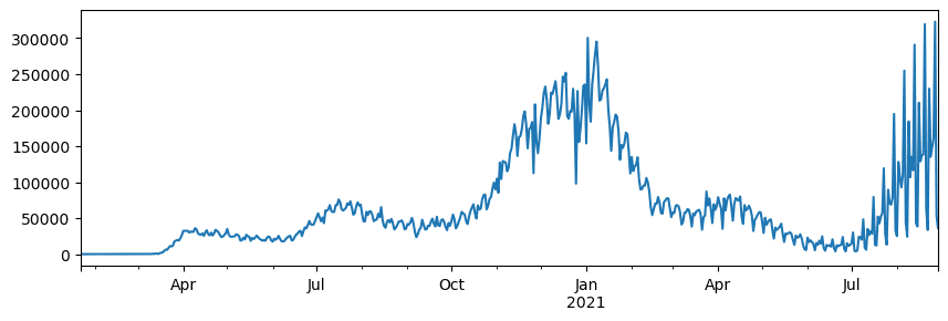
5.3.5.1. 🚀 Challenge 1: analyzing COVID spread#
First problem we will focus on is modelling of epidemic spread of COVID-19. In order to do that, we will use the data on the number of infected individuals in different countries, provided by the Center for Systems Science and Engineering (CSSE) at Johns Hopkins University. Dataset is available in this GitHub Repository.
Since we want to demonstrate how to deal with data, we invite you to open Estimation of COVID-19 pandemic and read it from top to bottom. You can also execute cells, and do some challenges that we have left for you at the end.
5.3.5.2. Working with unstructured Data#
While data very often comes in tabular form, in some cases we need to deal with less structured data, for example, text or images. In this case, to apply data processing techniques we have seen above, we need to somehow extract structured data. Here are a few examples:
Extracting keywords from text, and seeing how often those keywords appear
Using neural networks to extract information about objects on the picture
Getting information on emotions of people on video camera feed
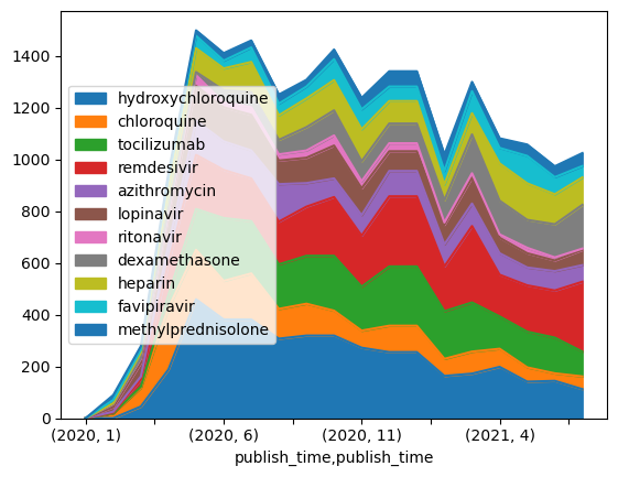
5.3.5.3. 🚀 Challenge 2: analyzing COVID papers#
In this challenge, we will continue with the topic of COVID pandemic, and focus on processing scientific papers on the subject. There is CORD-19 Dataset with more than 7000 (at the time of writing) papers on COVID, available with metadata and abstracts (and for about half of them there is also full text provided).
A full example of analyzing this dataset using Text Analytics for Health cognitive service is described in this blog post. We will discuss simplified version of this analysis.
Note
We do not provide a copy of the dataset as part of this repository. You may first need to download the metadata.csv file from this dataset on Kaggle. Registration with Kaggle may be required. You may also download the dataset without registration from here, but it will include all full texts in addition to metadata file.
Open Analyzing COVID-19 papers and read it from top to bottom. You can also execute cells, and do some challenges that we have left for you at the end.
5.3.6. Self study#
Books
Online resources
Official 10 minutes to Pandas tutorial
Learning Python
5.3.7. Acknowledgments#
Thanks for NumPy user guide. It contributes the introduction to NumPy.
Thanks to Microsoft for creating the open source course Data Science for Beginners. It contributes assignment section in this chapter.