Gradient descent
Contents
# Install the necessary dependencies

import sys
import os
!{sys.executable} -m pip install --quiet matplotlib numpy pandas ipython jupyterlab_myst scikit-learn
import matplotlib
import numpy as np
import pandas as pd
import sklearn
import matplotlib.pyplot as plt
from sklearn.model_selection import train_test_split
from IPython.display import HTML
13.2. Gradient descent#
13.2.1. Objective of this session#
We have already learnt how to use Linear Regression and Logistic Regression models.
The code might seem quite easy and intuitive for you. And you might naturally ask:
What’s behind the
.fit()function?Why sometimes it takes quite a bit for this
.fit()function to finish running?
In this session, you will learn that the .fit() is the training of ML models,
i.e. tuning of parameters for ML models. And the technique behind is called “Gradient Descent”.
13.2.2. Video#
The corresponding video (in Chinese) for this notebook is 👉 available here on Bilibili. You can (and should) watch the video before diving into the details of gradient descent:
from IPython.display import HTML

display(
    HTML(
        """
<p style="text-align: center;">
<iframe src="https://player.bilibili.com/player.html?aid=642485873&cid=764796592&page=1&high_quality=1&danmaku=0" width="105%" height="700px;" style="border:none;"></iframe>
video. <a href="https://player.bilibili.com/player.html?aid=642485873&cid=764796592&page=1&high_quality=1&danmaku=0">[source]</a>
</p>
"""
    )
)
video. [source]
13.2.3. Let’s be playful … to gain some intuition#
13.2.4. Some mathematics … to gain more insight#
13.2.4.1. Abstract#
The idea behind gradient descent is simple - by gradually tuning parameters, such as slope (\(m\)) and the intercept (\(b\)) in our regression function \(y = mx + b\), we minimize cost.
By cost, we usually mean some kind of a function that tells us how far off our model predicted result. For regression problems we often use mean squared error (MSE) cost function. If we use gradient descent for the classification problem, we will have a different set of parameters to tune.
Now we have to figure out how to tweak parameters \(m\) and \(b\) to reduce MSE.
13.2.4.2. Partial derivatives#
We use partial derivatives to find how each individual parameter affects MSE, so that’s where word partial comes from. In simple words, we take the derivative with respect to \(m\) and \(b\) separately. Take a look at the formula below. It looks almost exactly the same as MSE, but this time we added f(m, b) to it. It essentially changes nothing, except now we can plug \(m\) and \(b\) numbers into it and calculate the result.
This formula (or better say function) is better representation for further calculations of partial derivatives. We can ignore sum for now and what comes before that and focus only on \(y - (mx + b)^2\).
13.2.4.3. Partial derivative with respect to \(m\)#
With respect to \(m\) means we derive parameter \(m\) and basically ignore what is going on with \(b\), or we can say its 0. To derive with respect to \(m\) we will use chain rule.
Chain rule applies when one function sits inside of another. If you’re new to this, you’d be surprised that \(()^2\) is outside function, and \(y-(\boldsymbol{m}x+b)\) sits inside it. So, the chain rule says that we should take a derivative of outside function, keep inside function unchanged and then multiply by derivative of the inside function. Lets write these steps down:
Derivative of \(()^2\) is \(2()\), same as \(x^2\) becomes \(2x\)
We do nothing with \(y - (mx + b)\), so it stays the same
Derivative of \(y - (mx + b)\) with respect to m is \((0 - (x + 0))\) or \(-x\), because y and b are constants, they become 0, and derivative of mx is x
Multiply all parts we get following: \(2 * (y - (mx+b)) * -x\).
Looks nicer if we move -x to the left: \(-2x *(y-(mx+b))\). There we have it. The final version of our derivative is the following:
Here, \(\frac{df}{dm}\) means we find partial derivative of function f (we mentioned it earlier) with respect to m. We plug our derivative to the summation and we’re done.
13.2.4.4. Partial derivative with respect to \(b\)#
Same rules apply to the derivative with respect to b.
\(()^2\) becomes \(2()\), same as \(x^2\) becomes \(2x\)
\(y - (mx + b)\) stays the same
\(y - (mx + b)\) becomes \((0 - (0 + 1))\) or \(-1\), because y and mx are constants, they become 0, and derivative of b is 1
Multiply all the parts together and we get \(-2(y-(mx+b))\)
13.2.4.5. Final function#
Few details we should discuss before jumping into code:
Gradient descent is an iterative process and with each iteration (\(epoch\)) we slightly minimizing MSE, so each time we use our derived functions to update parameters \(m\) and \(b\).
Because it’s iterative, we should choose how many iterations we take, or make algorithm stop when we approach minima of MSE. In other words when algorithm is no longer improving MSE, we know it reached minimum.
Gradient descent has an additional parameter learning rate (\(lr\)), which helps control how fast or slow algorithm going towards minima of MSE
That’s about it. So you can already understand that Gradient Descent for the most part is just process of taking derivatives and using them over and over to minimize function.
13.2.5. Time to code!#
13.2.5.1. Linear regression With gradient descent#
class LinearRegression:
    def __init__(self, learning_rate=0.0003, n_iters=3000):
        self.lr = learning_rate
        self.n_iters = n_iters
        self.weights = None
        self.bias = None

    def fit(self, X, y):
        n_samples, n_features = X.shape

        # init parameters
        self.weights = np.zeros(n_features)
        self.bias = 0

        # gradient descent
        for _ in range(self.n_iters):
            # approximate y with linear combination of weights and x, plus bias
            y_predicted = np.dot(X, self.weights) + self.bias

            # compute gradients
            dw = (1 / n_samples) * np.dot(X.T, (y_predicted - y))
            db = (1 / n_samples) * np.sum(y_predicted - y)
            # update parameters
            self.weights -= self.lr * dw
            self.bias -= self.lr * db

    def predict(self, X):
        y_predicted = np.dot(X, self.weights) + self.bias
        return y_predicted
prostate = pd.read_table(
"https://static-1300131294.cos.ap-shanghai.myqcloud.com/data/ml-fundamental/parameter-optimization/gradient-descent/prostate.data"
)
prostate.drop(prostate.columns[0], axis=1, inplace=True)
X = prostate.drop(["lpsa", "train"], axis=1)
y = prostate["lpsa"]
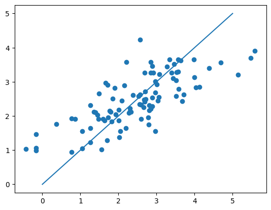
regressor = LinearRegression()
regressor.fit(X, y)
y_pred = regressor.predict(X)
print(regressor.__dict__)
print(y - y_pred)
plt.scatter(y, y_pred)
plt.plot([0, 5], [0, 5])
plt.show()
{'lr': 0.0003, 'n_iters': 3000, 'weights': array([0.36114314, 0.15172482, 0.01138062, 0.07103796, 0.10143793,
       0.14812986, 0.09146885, 0.00270041]), 'bias': 0.014542612245156494}
0    -1.470137
1    -1.226722
2    -1.633534
3    -1.145394
4    -1.385705
        ...
92    0.985388
93    1.125408
94    1.936285
95    1.776223
96    1.680470
Name: lpsa, Length: 97, dtype: float64
class LinearRegressionWithSGD:
    def __init__(self, learning_rate=0.0003, n_iters=5000):
        self.lr = learning_rate
        self.n_iters = n_iters
        self.weights = None
        self.bias = None

    def fit(self, X, y):
        n_samples, n_features = X.shape

        # init parameters
        self.weights = np.zeros(n_features)
        self.bias = 0

        batch_size = 5
        # stochastic gradient descent
        for _ in range(self.n_iters):
            # approximate y with linear combination of weights and x, plus bias
            y_predicted = np.dot(X, self.weights) + self.bias

            indexes = np.random.randint(0, len(X), batch_size)  # random sample

            Xs = np.take(X, indexes, axis=0)
            ys = np.take(y, indexes, axis=0)
            y_predicted_s = np.take(y_predicted, indexes)

            # compute gradients
            dw = (1 / batch_size) * np.dot(Xs.T, (y_predicted_s - ys))
            db = (1 / batch_size) * np.sum(y_predicted_s - ys)
            # update parameters
            self.weights -= self.lr * dw
            self.bias -= self.lr * db

    def predict(self, X):
        y_predicted = np.dot(X, self.weights) + self.bias
        return y_predicted
prostate = pd.read_table(
"https://static-1300131294.cos.ap-shanghai.myqcloud.com/data/ml-fundamental/parameter-optimization/gradient-descent/prostate.data"
)
prostate.drop(prostate.columns[0], axis=1, inplace=True)
X = prostate.drop(["lpsa", "train"], axis=1)
y = prostate["lpsa"]
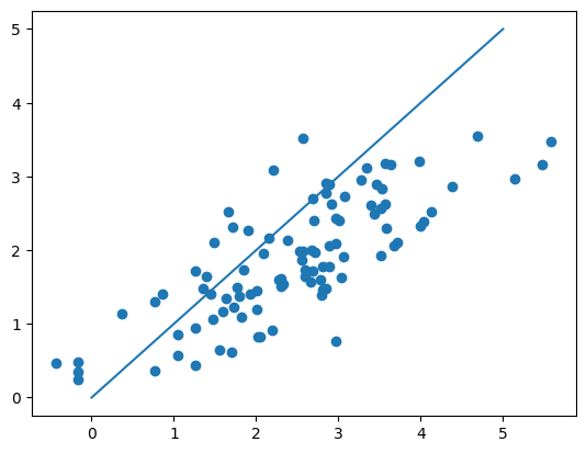
regressor = LinearRegressionWithSGD()
regressor.fit(X, y)
y_pred = regressor.predict(X)
print(regressor.__dict__)
print(y - y_pred)
plt.scatter(y, y_pred)
plt.plot([0, 5], [0, 5])
plt.show()
{'lr': 0.0003, 'n_iters': 5000, 'weights': array([ 0.45399277,  0.21512061, -0.00621535,  0.08132809,  0.14159593,
        0.13520515,  0.12171566,  0.00136173]), 'bias': 0.020739011982998982}
0    -0.903404
1    -0.515619
2    -0.649418
3    -0.412483
4    -0.773451
        ...
92    1.526965
93    1.135569
94    2.167430
95    2.318971
96    2.104345
Name: lpsa, Length: 97, dtype: float64
13.2.5.2. Logistic regression with gradient descent#
class LogisticRegression:
    def __init__(self, learning_rate=0.001, n_iters=1000):
        self.lr = learning_rate
        self.n_iters = n_iters
        self.weights = None
        self.bias = None

    def fit(self, X, y):
        n_samples, n_features = X.shape

        # init parameters
        self.weights = np.zeros(n_features)
        self.bias = 0

        # gradient descent
        for _ in range(self.n_iters):
            # approximate y with linear combination of weights and x, plus bias
            linear_model = np.dot(X, self.weights) + self.bias
            # apply sigmoid function
            y_predicted = self._sigmoid(linear_model)

            # compute gradients
            dw = (1 / n_samples) * np.dot(X.T, (y_predicted - y))
            db = (1 / n_samples) * np.sum(y_predicted - y)
            # update parameters
            self.weights -= self.lr * dw
            self.bias -= self.lr * db

    def predict(self, X):
        linear_model = np.dot(X, self.weights) + self.bias
        y_predicted = self._sigmoid(linear_model)
        y_predicted_cls = [1 if i > 0.5 else 0 for i in y_predicted]
        return np.array(y_predicted_cls)

    def _sigmoid(self, x):
        return 1 / (1 + np.exp(-x))
heart = pd.read_csv(
    "https://static-1300131294.cos.ap-shanghai.myqcloud.com/data/ml-fundamental/parameter-optimization/gradient-descent/SA_heart.csv"
)
heart.famhist.replace(to_replace=["Present", "Absent"], value=[1, 0], inplace=True)
heart.drop(["row.names"], axis=1, inplace=True)
X = heart.iloc[:, :-1]
y = heart.iloc[:, -1]

X_train, X_test, y_train, y_test = train_test_split(
    X, y, test_size=0.33, random_state=42
)

regressor = LogisticRegression(learning_rate=0.0001, n_iters=1000)

regressor.fit(X_train, y_train)
y_pred = regressor.predict(X_test)
perf = sklearn.metrics.confusion_matrix(y_test, y_pred)
print("LR classification perf:\n", perf)

error_rate = np.mean(y_test != y_pred)
print("LR classification error rate:\n", error_rate)
LR classification perf:
 [[88  9]
 [40 16]]
LR classification error rate:
 0.3202614379084967
13.2.6. Your turn 🚀#
Modify LogisticRegression so that the training will use SGD instead of GD.
13.2.7. [optional] At the frontier of Machine Learning Research#
from IPython.display import HTML

display(
    HTML(
        """
<p style="text-align: center;">
<iframe src="https://www.youtube.com/embed/mdKjMPmcWjY" width="105%" height="700px;" style="border:none;"></iframe>
video. <a href="https://www.youtube.com/embed/mdKjMPmcWjY">[source]</a>
</p>
"""
    )
)
video. [source]