# Install the necessary dependencies

import os
import sys
!{sys.executable} -m pip install --quiet seaborn pandas scikit-learn numpy matplotlib jupyterlab_myst ipython

37. Model training & evaluation

Machine Learning modeling, including model selection, training, evaluation and debugging, is very important, but only a small component of the entire Machine Learning pipeline. Some might even argue that it’s the easiest component. Details of specific algorithms won’t be discussed in this section. Instead, we will focus on giving an overview picture of how to choose the right model for the problem.

37.1. Model selection

Once problems are framed as one of the common Machine Learning tasks, the typical approaches to solve them can usually be located correspondingly. You should first figure out the category of the problem. Is it supervised or unsupervised? Or regression vs. classification? Does it require generation or only prediction? If it is the former, the models will have to be much harder to learn the latent space of the data.

Note that the model selection also highly depends on how the business problem is defined. For the same problem area, such as a house price prediction task, different targets may result in choosing different Machine Learning models. It can be regression if the required output is raw numbers. But if the goal is to quantize the income into different brackets and predict the bracket, it becomes a classification problem. Similarly, unsupervised learning could be used to learn labels for the data, which could be then used for supervised learning.

Keep in mind that there could be many ways to frame a problem, and the better one could only be known after the chosen models are trained and evaluated. Even though there are hundreds of ways to select and train a Machine Learning model, it is always a good practice to start with simple data, simple feature engineering, and simple model. Besides, transfer learning could be leveraged to reduce the training time in the context of the neural network. Furthermore, AutoML helps to further save time spent from feature engineering to HPO tuning. We will discuss these three useful tricks for selecting models in detail.

37.1.1. Start simple

When searching for a solution, the first goal is to find an effective simple approach for the task. This serves three major purposes.

• Focus on resolving the confidence about if the model could solve the problem, as additional complexity and potential bugs are avoided.

• Speed up the project iteration, and more complex components could be gradually added and verified step by step.

• At last, it is important to leverage the simplest solution to build up a reasonable baseline for further comparison with the comprehensive model.

“If you think that machine learning will give you a 100% boost, then a heuristic will get you 50% of the way there.” – Martin Zinkevich, research scientist at Google

See also

Martin, Z. (n.d.). Rules of machine learning: Best practices for ml engineering.

Start simple is about the architecture overall, which does a decent job on the problem. One or more aspects from below could be considered.

1. Simple data – start with the partial dataset if necessary, and easy-to-understand features which are easy to be captured by the model.

2. Simple processing - start with no regularization, normalization or other data processing as they may introduce bugs.

3. Simple model – start with a less complex model with sensible defaults, prove the feasibility, get a baseline, iterate and improve it gradually.

4. Simple problem - simplify the problem itself if possible, or achieve it in multiple steps or through several sub-problems.

For example, to simply start a house pricing prediction problem, firstly you could consider the most relevant features or a small portion of the data to build a simple linear regression model to get a baseline. Then you could add more features or data to extend the model to a nonlinear model. Or you could try other regressors such as decision trees, ensembles, shallow to deeper neural networks, etc, depending on the type and volume of data.

Overall, there is no need to pursue the state-of-the-art approach or the most optimized performance at the very beginning. But it is necessary to keep the eyes on the trap of increasingly complex heuristics.

37.1.2. Transfer learning

Transfer learning is a research problem in Machine Learning that focuses on storing knowledge gained while solving one problem and applying it to a different but related problem.

Using a large amount of data and tackling a completely new Machine Learning problem can be very challenging sometimes. Transfer learning could be the starting point if the simplified solution does not work or perform well. It allows utilizing knowledge(model) acquired (trained) for one task to solve other similar tasks.

What’s more, transfer learning is very commonly adopted in hot areas such as computer vision and natural language processing. It usually gives significantly better performance than training a simple model. And it is even a rare case to train a model from scratch in such areas. Instead, researchers and data scientists prefer starting from a pre-trained model that already learned general features and how to classify objects.

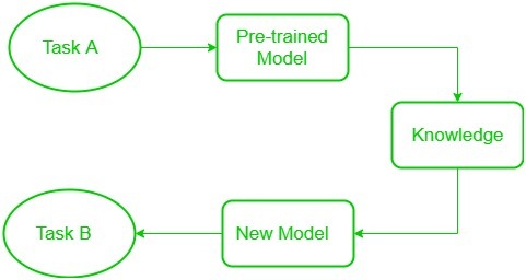
Fig. 37.1 Transfer learning

Traditionally, there are three major categories of transfer learning strategies and techniques based on the characteristics of the problem and the data. Inductive transfer learning is used if the domains are the same between the source and target, but the exact tasks are not. If the problems’ domains are even different, transductive transfer learning could be the choice. Unsupervised transfer learning is similar to inductive transfer learning, but for unsupervised tasks with unlabeled datasets both in the source and target.

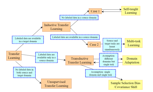
Fig. 37.2 Transfer learning strategies

Under the deep learning context, there are multiple levels of complexity in using a pre-trained model. The most straightforward way is to use the pre-trained model directly, but may not be applicable mostly. An idea here is to leverage the pre-trained model’s weighted layers to extract features while retraining the last layer. One step further, a more engaging technique is to fine-tune and train all layers after starting with only the feature layers. If it still does not work, fully training all the layers will be the fallback.

See also

What is transfer learning? [Examples & newbie-friendly guide]. (n.d.). Retrieved 27 July 2022.

37.1.3. AutoML

Automated Machine Learning(AutoML) provides methods and processes to make Machine Learning available for non-Machine Learning experts, to improve the efficiency of Machine Learning and accelerate research on Machine Learning. Designing and tuning Machine Learning systems is a labor and time-intensive task, and also requires extensive expertise. AutoML is focused on automating the model selection and training process.

As it is named, AutoML helps automate many aspects of Machine Learning model developments and training. It consists of a broader group of methodologies listed here:

• Automated Data Clean (Auto Clean)

• Automated Feature Engineering (Auto FE)

• Hyperparameter Optimization (HPO)

• Meta-Learning

• Neural Architecture Search (NAS)

Today, there are plenty of AutoML tools existing. It is important to understand the strengths and weaknesses of each other before going deep with any of them. AMLB provides an open and extensible benchmark to help compare and choose the right AutoML frameworks.

See also

Hutter, Frank, Lars Kotthoff, and Joaquin Vanschoren. Automated machine learning: methods, systems, challenges). Springer Nature, 2019.

37.2. Model evaluation

In practice, it is challenging to detect if the model is properly learning without under-fitting or overfitting. Ideally, before moving to production, it is always necessary to evaluate the trained model to make sure that everything is working properly. A common approach is to divide the dataset into three parts - training set, validation set and test set.

The model is trained by using only the train set, and the validation set is used to track the progress and conclude to optimize the model. Then the test set is used to evaluate the performance of the model. Using completely new data allows us to get an unbiased opinion on how well the algorithm works.

Fig. 37.3 Recommended method of dividing the data set

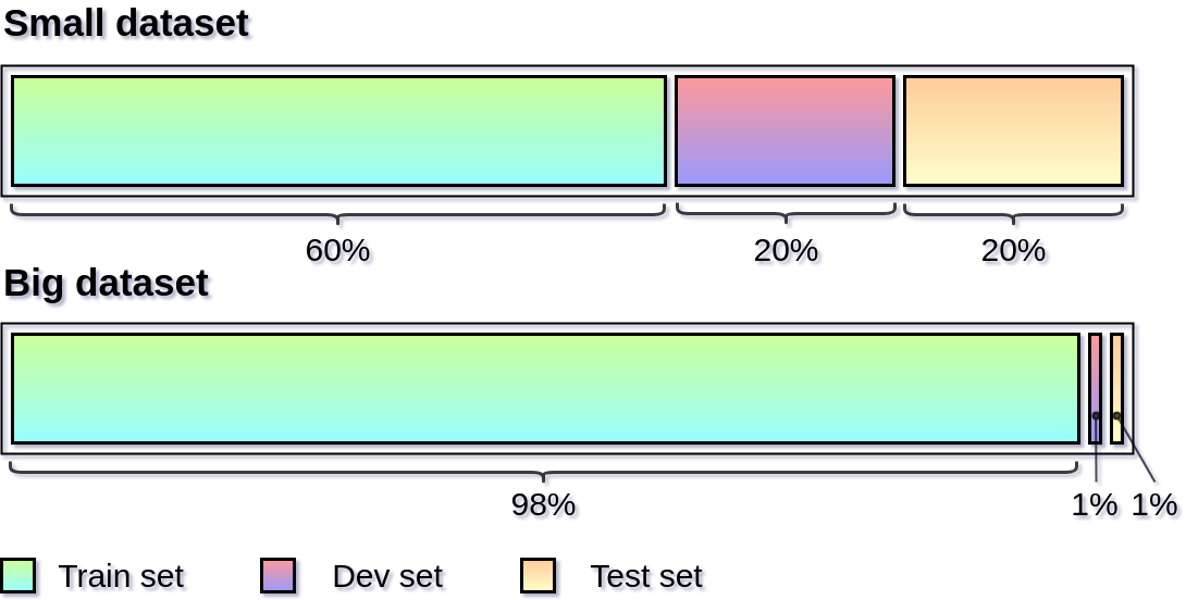
There is no strict heuristic about how to split the dataset, especially when working with big data. The split ratios depend greatly on the specific problem and data volume. Generally speaking, the train vs. validation vs. test split should allow for:

• Large enough validation set to compare the difference between models,

• Large enough test set to be representative of overall performance.

However, while evaluating a Machine Learning model can seem daunting, model metrics show where to start. The following sections discuss how to evaluate performance using metrics.

37.2.1. Evaluate quality using model metrics

To evaluate your model’s quality, commonly-used metrics are:

• loss

• accuracy

• precision & recall

• area under the ROC curve (AUC)

For guidance on interpreting these metrics, read the linked content from Machine Learning Crash Content. For additional guidance on specific problems, see the following table.

Problem	Evaluating Quality
Regression	Besides reducing the absolute Mean Square Error (MSE), reduce the MSE relative to the label values. For example, assume to predict prices of two items that have mean prices of 5 and 100. In both cases, assume the MSE is 5. In the first case, the MSE is 100% of your mean price, which is clearly a large error. In the second case, the MSE is 5% of the mean price, which is a reasonable error.
Multiclass classification	To predict a small number of classes, look at per-class metrics individually. When predicting on many classes, the per-class metrics can be leveraged to track overall classification metrics. Alternatively, specific quality goals can be prioritized depending on the needs. For example, if to classify objects in images, then the classification quality may be prioritized for people over other objects.
Ranking metrics	MRR, MAR, ordered logit
Computer vision	IoU, Pixel Accuracy
NLP	Perplexity, BLEU, ROUGE

Ideally, choose one single metric to optimize at once; if the requirement is to include multiple metrics, then consider a unified metric.

However, since the real world does not always go as what is imagined, it may be the case to try many metrics before finding one that could be satisfied with, and the metrics may change alongside the development, or even after getting the model into production.

37.2.2. Check metrics for important data slices

After having a high-quality model, the model might still perform poorly on subsets of the data. For example, the unicorn predictor must predict well both in the Sahara desert and in New York City, and at all times of the day. However, there is less training data for the Sahara desert. Therefore, it is necessary to track model quality specifically for the Sahara desert. Such subsets of data, like the subset corresponding to the Sahara desert, are called data slices. Data slices should be separately monitored where performance is especially important or where the model might perform poorly.

Use the understanding of the data to identify data slices of interest. Then compare model metrics for data slices against the metrics for the entire data set. Checking that the model performs across all data slices helps remove bias. For more, see Fairness: Evaluating for Bias.

37.2.3. Use real-world metrics

Model metrics do not necessarily measure the real-world impact of the model. For example, the AUC could be increased by changing a hyperparameter, but how did the change affect the user experience? To measure real-world impact, separate metrics need to be defined. Measuring real-world impact helps compare the quality of different iterations of the model.

37.2.4. Optimizing and satisfying metrics

As models are getting bigger and more resource-intensive, how to scale the mode training becomes more and more important. Thinking beyond the above model metrics, the model utilitarian performance should also be considered. It includes the training speed, inference speed, model size, model stability, etc.

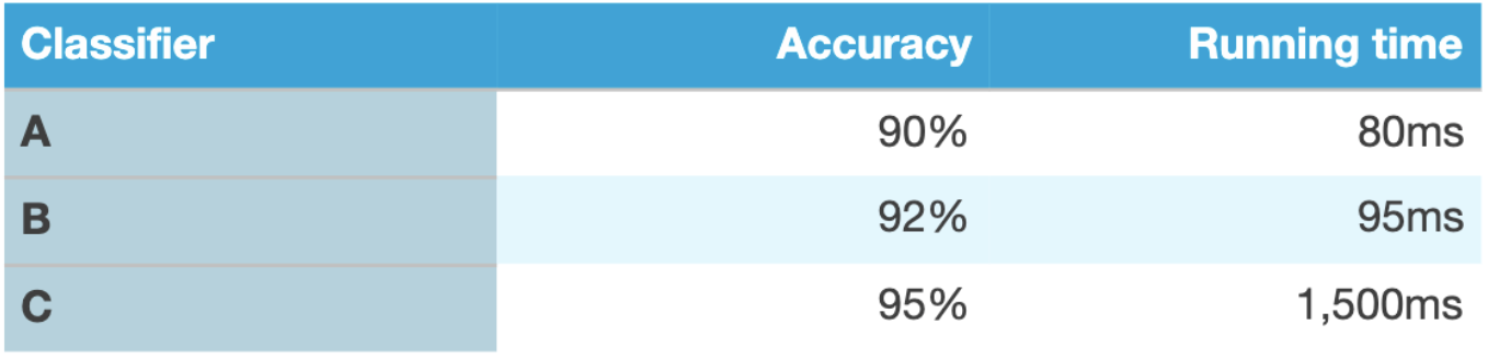
To the given example ng2017mlyearning below, both model accuracy and running time are important to decide which is the best classifier. It may not be natural to derive a single metric from them. Instead, a more real-world thinking-based strategy could be applied. The running time is important, but mostly it could be acceptable once under a certain value, such as 100ms. Whenever this condition is satisfied and the running time is good enough for production, then accuracy needs to be optimized with the best effort. Here, the running time is the satisfying metric and the accuracy is the optimizing metric.

Optimizing and satisfying metrics could also be applied to evaluate the model among different model metrics. As a final example, to build a natural language processing powered smart speaker’s device like Alexa, the wake word detection module is the key to support using a microphone to listen for the user saying a particular “wake-word” to wake up the system, such as the “Alexa” for Amazon Echo.

The false positive rate is one of the key metrics, which is about the frequency of the system waking up even when no one says the wake-word. While the false negative rate describes how often it fails to wake up when someone says the wake-word. It is difficult to optimize both of them at the same time. Instead, one reasonable way is to have the false negative rate as the optimizing metric which needs to be minimized. And the false positive could be treated as the satisfying metric, which should happen no more than once every 24 hours of operation.

37.3. Model debugging & improvement

Once the model is working, the next step is to optimize the model’s quality for production readiness. Both debugging and optimizing are critical in the Machine Learning pipeline.

How is Machine Learning debugging different? Before diving into any particular Machine Learning debugging method, it is important to understand what differentiates debugging Machine Learning models from traditional software programs. Unlike the latter, an Machine Learning model with poor quality usually does not imply the presence of a bug. Instead, There could be many reasons to cause a model not to perform well. So that to debug poor performance in a model, a broader range of potential causes need to be investigated compared to traditional programming.

For example, here are a few causes for poor model performance:

• Theoretical constraints, such as wrong assumptions, unsuccessful problem framing, and poor model/data fit.

• Data contains errors and anomalies or is over-preprocessed.

• Features lack predictive power.

• Poor feature engineering code contains bugs.

• Poor model implementation.

• Hyperparameters are set to non-optimal values.

Debugging Machine Learning models is complicated by the time it takes to run your experiments. Given the longer iteration cycles, and the larger error space, debugging Machine Learning models is uniquely challenging.

37.3.1. Data and feature debugging

Low-quality data will significantly affect your model’s performance. It’s much easier to detect low-quality data at input instead of guessing at its existence after the model predicts badly. Monitor the data by following the advice in this section.

Validate input data using rules.

To monitor the data, one approach is to write rules that the data must satisfy, and continuously check the data against the expected data quality. This collection of rules is defined by following these steps:

1. For the feature data, understand the range and distribution. For categorical features, understand the set of possible values.

2. Encode the understanding into rules. Examples of rules are:

   1. Ensure that user-submitted ratings are always between 1 and 5.

   2. Check that “the” occurs most frequently (for an English text feature).

   3. Check that categorical features have values from a fixed set.

3. Test the data against the rules which should catch data errors such as:

   1. anomalies.

   2. unexpected values of categorical variables.

   3. unexpected data distributions.

Ensure splits are good quality.

The test and training splits must be equally representative of the input data. If the test and training splits are statistically different, then training data will not help predict the test data. It’s often a struggle to gather enough data for a machine learning project. Sometimes, however, there is too much data, and a subset of examples must be selected for training.

Monitor the statistical properties of the splits. If the properties diverge, raise a flag. Further, test that the ratio of examples in each split stays constant. For example, if the data is split 80:20, that ratio should not change.

Test processed data.

While the raw data might be valid, the model only sees processed feature data. Because processed data looks very different from raw input data, it is necessary to check processed data separately. Based on the understanding of the processed data, write unit tests to verify if the data quality assurance is successfully applied through the data engineering process. For example, unit tests could check the following conditions:

1. All numeric features are scaled, for example, between 0 and 1.

2. One-hot encoded vectors only contain a single 1 and N-1 zeroes.

3. Missing data is replaced by mean or default values.

4. Data distributions after transformation conform to expectations. For example, if the data is normalized by using z-scores, the mean of the z-scores is 0.

5. Outliers are handled, such as by scaling or clipping.

37.3.2. Model debugging

After debugging the data, follow these steps to continue debugging the model.

Check that the model can predict labels.

Before debugging the model, try to determine whether the features encode predictive signals. Linear correlations could be found between individual features and labels by using correlation matrices.

However, correlation matrices will not detect nonlinear correlations between features and labels. Instead, choose 10 examples from the dataset that the model can easily learn from. Alternatively, use synthetic data that is easily learnable. For instance, a classifier can easily learn linearly-separable examples while a regressor can easily learn labels that correlate highly with a feature cross. Then, ensure the model can achieve a very small loss on these 10 easily-learnable examples.

Then using a few examples that are easily learnable simplifies debugging by reducing the opportunities for bugs. If it does not work well, consider to further simplifying the model by switching to the simpler gradient descent algorithm instead of a more advanced optimization algorithm.

Establish a baseline.

Comparing the model against a baseline is a quick test of the model’s quality. When developing a new model, define a baseline by using a simple heuristic to predict the label. If the trained model performs worse than its baseline, it needs to be improved.

Examples of baselines are:

• Using a linear model trained solely on the most predictive feature.

• In classification, always predict the most common label.

• In regression, always predicting the mean value.

Once a version of the model is validated in production, it could be used as a baseline for newer model versions. Therefore, there could be multiple baselines of different complexities. Testing against baselines helps justify adding complexity to the model. A more complex model should always perform better than a less complex model or baseline.

Implement tests for Machine Learning code.

The testing process to catch bugs in Machine Learning code is similar to the testing process in traditional debugging. Unit tests could be added to detect bugs. Examples of code bugs in Machine Learning are:

• Hidden layers that are configured incorrectly.

• Data normalization code that returns NaNs.

A sanity check for the presence of code bugs is to include the label in the features and train the model. If the model does not work, then it has a bug.

Adjust hyperparameter values.

The table below explains how to adjust values for the hyperparameters.

Hyperparameter	Description
Learning Rate	Typically, ML libraries will automatically set the learning rate. For example, in TensorFlow, most TF Estimators use the AdagradOptimizer, which sets the learning rate at 0.05 and then adaptively modifies the learning rate during training. The other popular optimizer, AdamOptimizer, uses an initial learning rate of 0.001. However, if your model does not converge with the default values, then manually choose a value between 0.0001 and 1.0, and increase or decrease the value on a logarithmic scale until your model converges. Remember that the more difficult your problem, the more epochs your model must train for before loss starts to decrease.
Regularization	First, ensure your model can predict without regularization on the training data. Then add regularization only if your model is overfitting on training data. Regularization methods differ for linear and nonlinear models. For linear models, choose L1 regularization if you need to reduce your model’s size. Choose L2 regularization if you prefer increased model stability. Increasing your model’s stability makes your model training more reproducible. Find the correct value of the regularization rate, , by starting at 1e-5 and tuning that value through trial and error. To regularize a deep neural network model, use Dropout regularization. Dropout removes a random selection of a fixed percentage of the neurons in a network layer for a single gradient step. Typically, dropout will improve generalization at a dropout rate of between 10% and 50% of neurons.
Training epochs	You should train for at least one epoch, and continue to train so long as you are not overfitting.
Batch size	Typically, the batch size of a mini-batch is between 10 and 1000. For SGD, the batch size is 1. The upper bound on your batch size is limited by the amount of data that can fit in your machine’s memory. The lower bound on batch size depends on your data and algorithm. However, using a smaller batch size lets your gradient update more often per epoch, which can result in a larger decrease in loss per epoch. Furthermore, models trained using smaller batches generalize better. For details, see On large-batch training for deep learning: Generalization gap and sharp minima N. S. Keskar, D. Mudigere, J. Nocedal, M. Smelyanskiy, and P. T. P. Tang. ICLR, 2017. Prefer using the smallest batch sizes that result in stable training.
Depth and width of layers	In a neural network, depth refers to the number of layers, and width refers to the number of neurons per layer. Increase depth and width as the complexity of the corresponding problem increases. Adjust your depth and width by following these steps: 1. Start with 1 fully-connected hidden layer with the same width as your input layer. 2. For regression, set the output layer’s width to 1. For classification, set the output layer’s width to the number of classes. 3. If your model does not work, and you think your model needs to be deeper to learn your problem, then increase depth linearly by adding a fully-connected hidden layer at a time. The hidden layer’s width depends on your problem. A commonly-used approach is to use the same width as the previous hidden layer, and then discover the appropriate width through trial-and-error. The change in width of successive layers also depends on your problem. A practice drawn from common observation is to set a layer’s width equal to or less than the width of the previous layer. Remember, the depth and width don’t have to be exactly right. You’ll tune their values later when you optimize your model.

37.3.3. Interpreting loss curves

Machine learning would be a breeze if all our loss curves looked like this the first time we trained our model:

But in reality, loss curves can be quite challenging to interpret. Use your understanding of loss curves to answer the following questions.

1. My model won’t train!

Your friend Mel and you continue working on a unicorn appearance predictor. Here’s your first loss curve.

Your model is not converging. Try these debugging steps:

• Check if your features can predict the labels by following the steps in Model debugging.

• Check your data against a rules to detect bad examples.

• If training looks unstable, as in this plot, then reduce your learning rate to prevent the model from bouncing around in parameter space.

• Simplify your dataset to 10 examples that you know your model can predict. Obtain a very low loss on the reduced dataset. Then continue debugging your model on the full dataset.

• Simplify your model and ensure the model outperforms your baseline. Then incrementally add complexity to the model.

2. My loss exploded!

Mel shows you another curve. What’s going wrong here and how can she fix it? Write your answer below.

A large increase in loss is typically caused by anomalous values in input data. Possible causes are:

• NaNs in input data.

• Exploding gradient due to anomalous data.

• Division by zero.

• Logarithm of zero or negative numbers.

To fix an exploding loss, check for anomalous data in your batches, and in your engineered data. If the anomaly appears problematic, then investigate the cause. Otherwise, if the anomaly looks like outlying data, then ensure the outliers are evenly distributed between batches by shuffling your data.

3. My metrics are contradictory!

Mel wants your take on another curve. What’s going wrong and how can she fix it? Write your answer below.

The recall is stuck at 0 because your examples’ classification probability is never higher than the threshold for positive classification. This situation often occurs in problems with a large class imbalance. Remember that ML libraries, such as TF Keras, typically use a default threshold of 0.5 to calculate classification metrics.

Try these steps:

• Lower your classification threshold.

• Check threshold-invariant metrics, such as AUC.

4. Testing loss is too damn high!

Mel shows you the loss curves for training and testing datasets and asks “What’s wrong?” Write your answer below.

Your model is overfitting to the training data. Try these steps:

• Reduce model capacity.

• Add regularization.

• Check that the training and test splits are statistically equivalent.

5. My model gets stuck.

You’re patient when Mel returns a few days later with yet another curve. What’s going wrong here and how can Mel fix it?

Your loss is showing repetitive, step-like behavior. The input data seen by your model probably is itself exhibiting repetitive behavior. Ensure that shuffling is removing repetitive behavior from input data.

It’s working!

“It’s working perfectly now!” Mel exclaims. She leans back into her chair triumphantly and heaves a big sigh. The curve looks great and you beam with accomplishment. Mel and you take a moment to discuss the following additional checks for validating your model.

• real-world metrics

• baselines

• absolute loss for regression problems

• other metrics for classification problems

37.4. Model optimization

Once the model is working, it’s time to optimize the model’s quality. Follow the steps below.

37.4.1. Add useful features

The model performance could be improved by adding features that encode information not yet encoded by the existing features. Correlation matrices could be used to find linear correlations between individual features and labels. To detect nonlinear correlations between features and labels, the model must be trained with and without the feature, or combination of features, and check for an increase in model quality. The feature’s inclusion must be justified by an increase in model quality.

37.4.2. Tune hyperparameters

Values of hyperparameters make your model work. However, these hyperparameter values can still be tuned. The values could be tuned manually by trial and error, but manual tuning is time-consuming. Instead, consider using an AutoML hyperparameter tuning service, such as Google Cloud Machine Learning hyperparameter tuning, Auto Gluon, etc. With different sets of hyperparameters, the same model may perform drastically differently on the same dataset. Keep in mind that not all hyperparameters are created equal. A model could be more sensitive to one hyperparameter.

37.4.3. Tune model depth and width

While debugging the model, its depth and width are increased to improve the model performance In contrast, during model optimization, the mode depth and width could be either increased or decreased depending on the goals. If the model quality is adequate, then try reducing overfitting and training time by decreasing depth and width. Specifically, try halving the width at each successive layer. Since the model quality will also decrease, it is always a trade-off to balance quality with overfitting and training time.

Conversely, if the goal is to have higher model quality, then try increasing depth and width. Remember that increases in depth and width are practically limited by accompanying increases in training time and overfitting. To understand overfitting.

Since depth and width are hyperparameters, hyperparameter tuning could be used to optimize depth and width.

37.5. Your turn! 🚀

Understanding the challenges in Machine Learning debugging by completing the Counterintuitive Challenges in ML Debugging.

Apply the debugging concepts learned by completing the following:

• Case Study: Debugging in Regression

• Case Study: Debugging in Classification

37.6. Self study

• Machine Learning Algorithms: Which One to Choose for Your Problem by Daniil Korbut, Stats and Bots, 2017.

37.7. Acknowledgments

Thanks to Google for creating the open-source course Testing and Debugging in Machine Learning which is licensed under CC-BY 4.0. It contributes to the majority of Model evaluation, Model debugging & improvement, Model optimization, and assignments.

Thanks to chiphuyen for creating the Machine Learning Systems Design which inspires some of the contents in this section.