42.94. How to choose cnn architecture mnist#

42.94.1. What is the best CNN architecture for MNIST?#

There are so many choices for CNN architecture. How do we choose the best one? First we must define what best means. The best may be the simplest, or it may be the most efficient at producing accuracy while minimizing computational complexity. In this kernel, we will run experiments to find the most accurate and efficient CNN architecture for classifying MNIST handwritten digits.

The best known MNIST classifier found on the internet achieves 99.8% accuracy!! That’s amazing. The best Kaggle kernel MNIST classifier achieves 99.75% [posted here][https://www.kaggle.com/cdeotte/25-million-images-0-99757-mnist]. This kernel demostrates the experiments used to determine that kernel’s CNN architecture.

42.94.2. Basic CNN structure#

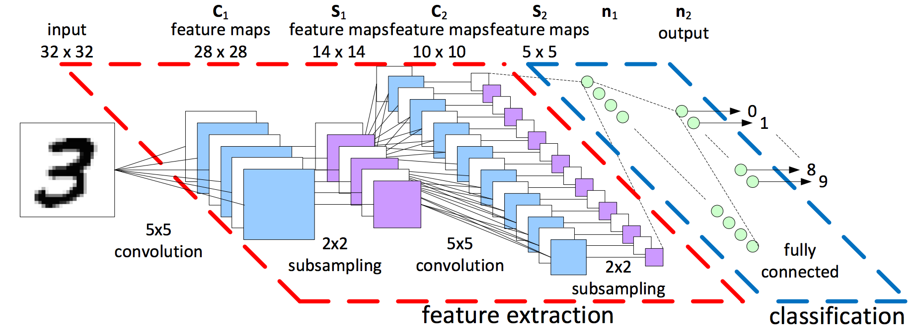
A typical CNN design begins with feature extraction and finishes with classification. Feature extraction is performed by alternating convolution layers with subsambling layers. Classification is performed with dense layers followed by a final softmax layer. For image classification, this architecture performs better than an entirely fully connected feed forward neural network. extract

42.94.3. Load libraries#

import pandas as pd
import numpy as np
from sklearn.model_selection import train_test_split
from keras.utils.np_utils import to_categorical
from keras.models import Sequential
from keras.layers import (
    Dense,
    Dropout,
    Flatten,
    Conv2D,
    MaxPool2D,
    AvgPool2D,
    BatchNormalization,
    Reshape,
)
from keras.preprocessing.image import ImageDataGenerator
from keras.callbacks import LearningRateScheduler
import matplotlib.pyplot as plt

42.94.4. Load the data#

train = pd.read_csv("https://static-1300131294.cos.ap-shanghai.myqcloud.com/data/deep-learning/cnn/mnist_train.csv")
test = pd.read_csv("https://static-1300131294.cos.ap-shanghai.myqcloud.com/data/deep-learning/cnn/mnist_test.csv")

42.94.5. Prepare data for neural network#

Y_train = train["label"]
X_train = train.drop(labels=["label"], axis=1)
X_train = X_train / 255.0

Y_test = test["label"]
X_test = test.drop(labels=["label"], axis=1)
X_test = X_test / 255.0

X_train = X_train.values.reshape(-1, 28, 28, 1)
X_test = X_test.values.reshape(-1, 28, 28, 1)
Y_train = to_categorical(Y_train, num_classes=10)
Y_test = to_categorical(Y_test, num_classes=10)

42.94.6. Global variables#

annealer = LearningRateScheduler(lambda x: 1e-3 * 0.95**x, verbose=0)
styles = [":", "-.", "--", "-", ":", "-.", "--", "-", ":", "-.", "--", "-"]

42.94.7. 1. How many convolution-subsambling pairs?#

First question, how many pairs of convolution-subsampling should we use? For example, our network could have 1, 2, or 3:

784 - [24C5-P2] - 256 - 10
784 - [24C5-P2] - [48C5-P2] - 256 - 10
784 - [24C5-P2] - [48C5-P2] - [64C5-P2] - 256 - 10

It’s typical to increase the number of feature maps for each subsequent pair as shown here.

42.94.8. Experiment 1#

Let’s see whether one, two, or three pairs is best. We are not doing four pairs since the image will be reduced too small before then. The input image is 28x28. After one pair, it’s 14x14. After two, it’s 7x7. After three it’s 4x4 (or 3x3 if we don’t use padding=‘same’). It doesn’t make sense to do a fourth convolution.

42.94.8.1. Build convolutional neural networks#

nets = 3
model = [0] * nets

for j in range(3):
    model[j] = Sequential()
    model[j].add(
        Conv2D(
            24,
            kernel_size=5,
            padding="same",
            activation="relu",
            input_shape=(28, 28, 1),
        )
    )
    model[j].add(MaxPool2D())
    if j > 0:
        model[j].add(Conv2D(48, kernel_size=5, padding="same", activation="relu"))
        model[j].add(MaxPool2D())
    if j > 1:
        model[j].add(Conv2D(64, kernel_size=5, padding="same", activation="relu"))
        model[j].add(MaxPool2D(padding="same"))
    model[j].add(Flatten())
    model[j].add(Dense(256, activation="relu"))
    model[j].add(Dense(10, activation="softmax"))
    model[j].compile(
        optimizer="adam", loss="categorical_crossentropy", metrics=["accuracy"]
    )

42.94.8.2. Create validation set and train networks#

X_train2, X_val2, Y_train2, Y_val2 = train_test_split(X_train, Y_train, test_size=0.333)
history = [0] * nets
names = ["(C-P)x1", "(C-P)x2", "(C-P)x3"]
epochs = 30
for j in range(nets):
    history[j] = model[j].fit(
        X_train2,
        Y_train2,
        batch_size=80,
        epochs=epochs,
        validation_data=(X_val2, Y_val2),
        callbacks=[annealer],
        verbose=0,
    )
    print(
        "CNN {0}: Epochs={1:d}, Train accuracy={2:.5f}, Validation accuracy={3:.5f}".format(
            names[j],
            epochs,
            max(history[j].history["accuracy"]),
            max(history[j].history["val_accuracy"]),
        )
    ) 

42.94.8.3. Plot accuracies#

plt.figure(figsize=(15, 5))
for i in range(nets):
    plt.plot(history[i].history["val_accuracy"], linestyle=styles[i])
plt.title("model accuracy")
plt.ylabel("accuracy")
plt.xlabel("epoch")
plt.legend(names, loc="upper left")
axes = plt.gca()
axes.set_ylim([0.9, 1])
plt.show()

42.94.8.4. Summary#

From the above experiment, it seems that 3 pairs of convolution-subsambling is slightly better than 2 pairs. However for efficiency, the improvement doesn’t warrant the additional computional cost, so let’s use 2.

42.94.9. 2. How many feature maps?#

In the previous experiement, we decided that two pairs is sufficient. How many feature maps should we include? For example, we could do

784 - [8C5-P2] - [16C5-P2] - 256 - 10
784 - [16C5-P2] - [32C5-P2] - 256 - 10
784 - [24C5-P2] - [48C5-P2] - 256 - 10
784 - [32C5-P2] - [64C5-P2] - 256 - 10
784 - [48C5-P2] - [96C5-P2] - 256 - 10
784 - [64C5-P2] - [128C5-P2] - 256 - 10

42.94.10. Experiment 2#

42.94.10.1. Build convolutional neural networks#

nets = 6
model = [0] * nets
for j in range(6):
    model[j] = Sequential()
    model[j].add(
        Conv2D(j * 8 + 8, kernel_size=5, activation="relu", input_shape=(28, 28, 1))
    )
    model[j].add(MaxPool2D())
    model[j].add(Conv2D(j * 16 + 16, kernel_size=5, activation="relu"))
    model[j].add(MaxPool2D())
    model[j].add(Flatten())
    model[j].add(Dense(256, activation="relu"))
    model[j].add(Dense(10, activation="softmax"))
    model[j].compile(
        optimizer="adam", loss="categorical_crossentropy", metrics=["accuracy"]
    )

42.94.10.2. Create validation set and train networks#

X_train2, X_val2, Y_train2, Y_val2 = train_test_split(X_train, Y_train, test_size=0.333)
history = [0] * nets
names = ["8 maps", "16 maps", "24 maps", "32 maps", "48 maps", "64 maps"]
epochs = 30
for j in range(nets):
    history[j] = model[j].fit(
        X_train2,
        Y_train2,
        batch_size=80,
        epochs=epochs,
        validation_data=(X_val2, Y_val2),
        callbacks=[annealer],
        verbose=0,
    )
    print(
        "CNN {0}: Epochs={1:d}, Train accuracy={2:.5f}, Validation accuracy={3:.5f}".format(
            names[j],
            epochs,
            max(history[j].history["accuracy"]),
            max(history[j].history["val_accuracy"]),
        )
    )

42.94.10.3. Plot accuracies#

plt.figure(figsize=(15, 5))
for i in range(nets):
    plt.plot(history[i].history["val_accuracy"], linestyle=styles[i])
plt.title("model accuracy")
plt.ylabel("accuracy")
plt.xlabel("epoch")
plt.legend(names, loc="upper left")
axes = plt.gca()
axes.set_ylim([0.9, 1])
plt.show()

42.94.10.4. Summary#

From the above experiement, it appears that 32 maps in the first convolutional layer and 64 maps in the second convolutional layer is the best. Architectures with more maps only perform slightly better and are not worth the additonal computation cost.

42.94.11. 3. How large a dense layer?#

In our previous experiment, we decided on 32 and 64 maps in our convolutional layers. How many dense units should we use? For example we could use

784 - [32C5-P2] - [64C5-P2] - 0 - 10
784 - [32C5-P2] - [64C5-P2] - 32 - 10
784 - [32C5-P2] - [64C5-P2] - 64 - 10
784 - [32C5-P2] - [64C5-P2] - 128 -10
784 - [32C5-P2] - [64C5-P2] - 256 - 10
784 - [32C5-P2] - [64C5-P2] - 512 -10
784 - [32C5-P2] - [64C5-P2] - 1024 - 10
784 - [32C5-P2] - [64C5-P2] - 2048 - 10

42.94.12. Experiment 3#

42.94.13. Build convolutional neural networks#

nets = 8
model = [0] * nets

for j in range(8):
    model[j] = Sequential()
    model[j].add(Conv2D(32, kernel_size=5, activation="relu", input_shape=(28, 28, 1)))
    model[j].add(MaxPool2D())
    model[j].add(Conv2D(64, kernel_size=5, activation="relu"))
    model[j].add(MaxPool2D())
    model[j].add(Flatten())
    if j > 0:
        model[j].add(Dense(2 ** (j + 4), activation="relu"))
    model[j].add(Dense(10, activation="softmax"))
    model[j].compile(
        optimizer="adam", loss="categorical_crossentropy", metrics=["accuracy"]
    )

42.94.14. Create validation set and train networks#

X_train2, X_val2, Y_train2, Y_val2 = train_test_split(X_train, Y_train, test_size=0.333)

history = [0] * nets
names = ["0N", "32N", "64N", "128N", "256N", "512N", "1024N", "2048N"]
epochs = 30
for j in range(nets):
    history[j] = model[j].fit(
        X_train2,
        Y_train2,
        batch_size=80,
        epochs=epochs,
        validation_data=(X_val2, Y_val2),
        callbacks=[annealer],
        verbose=0,
    )
    print(
        "CNN {0}: Epochs={1:d}, Train accuracy={2:.5f}, Validation accuracy={3:.5f}".format(
            names[j],
            epochs,
            max(history[j].history["accuracy"]),
            max(history[j].history["val_accuracy"]),
        )
    )

42.94.15. Plot accuracies#

plt.figure(figsize=(15, 5))
for i in range(nets):
    plt.plot(history[i].history["val_accuracy"], linestyle=styles[i])
plt.title("model accuracy")
plt.ylabel("accuracy")
plt.xlabel("epoch")
plt.legend(names, loc="upper left")
axes = plt.gca()
axes.set_ylim([0.9, 1])
plt.show()

42.94.15.1. Summary#

From this experiment, it appears that 128 units is the best. Dense layers with more units only perform slightly better and are not worth the additional computational cost. (We also tested using two consecutive dense layers instead of one, but that showed no benefit over a single dense layer.)

42.94.16. 4. How much dropout?#

Dropout will prevent our network from overfitting thus helping our network generalize better. How much dropout should we add after each layer?

0%, 10%, 20%, 30%, 40%, 50%, 60%, or 70%

42.94.17. Experiment 4#

42.94.18. Build convolutional neural networks#

nets = 8
model = [0] * nets

for j in range(8):
    model[j] = Sequential()
    model[j].add(Conv2D(32, kernel_size=5, activation="relu", input_shape=(28, 28, 1)))
    model[j].add(MaxPool2D())
    model[j].add(Dropout(j * 0.1))
    model[j].add(Conv2D(64, kernel_size=5, activation="relu"))
    model[j].add(MaxPool2D())
    model[j].add(Dropout(j * 0.1))
    model[j].add(Flatten())
    model[j].add(Dense(128, activation="relu"))
    model[j].add(Dropout(j * 0.1))
    model[j].add(Dense(10, activation="softmax"))
    model[j].compile(
        optimizer="adam", loss="categorical_crossentropy", metrics=["accuracy"]
    )

42.94.19. Create validation set and train networks#

X_train2, X_val2, Y_train2, Y_val2 = train_test_split(X_train, Y_train, test_size=0.333)

history = [0] * nets
names = ["D=0", "D=0.1", "D=0.2", "D=0.3", "D=0.4", "D=0.5", "D=0.6", "D=0.7"]
epochs = 30
for j in range(nets):
    history[j] = model[j].fit(
        X_train2,
        Y_train2,
        batch_size=80,
        epochs=epochs,
        validation_data=(X_val2, Y_val2),
        callbacks=[annealer],
        verbose=0,
    )
    print(
        "CNN {0}: Epochs={1:d}, Train accuracy={2:.5f}, Validation accuracy={3:.5f}".format(
            names[j],
            epochs,
            max(history[j].history["accuracy"]),
            max(history[j].history["val_accuracy"]),
        )
    )

42.94.20. Plot accuracies#

plt.figure(figsize=(15, 5))
for i in range(nets):
    plt.plot(history[i].history["val_accuracy"], linestyle=styles[i])
plt.title("model accuracy")
plt.ylabel("accuracy")
plt.xlabel("epoch")
plt.legend(names, loc="upper left")
axes = plt.gca()
axes.set_ylim([0.9, 1])
plt.show()

42.94.21. Summary#

From this experiment, it appears that 40% dropout is the best.

42.94.22. 5. Advanced features#

Instead of using one convolution layer of size 5x5, you can mimic 5x5 by using two consecutive 3x3 layers and it will be more nonlinear. Instead of using a max pooling layer, you can subsample by using a convolution layer with strides=2 and it will be learnable. Lastly, does batch normalization help? And does data augmentation help? Let’s test all four of these

replace ‘32C5’ with ‘32C3-32C3’
replace ‘P2’ with ‘32C5S2’
add batch normalization
add data augmentation

42.94.23. Build convolutional neural networks#

nets = 5
model = [0] * nets

j = 0
model[j] = Sequential()
model[j].add(Conv2D(32, kernel_size=5, activation="relu", input_shape=(28, 28, 1)))
model[j].add(MaxPool2D())
model[j].add(Dropout(0.4))
model[j].add(Conv2D(64, kernel_size=5, activation="relu"))
model[j].add(MaxPool2D())
model[j].add(Dropout(0.4))
model[j].add(Flatten())
model[j].add(Dense(128, activation="relu"))
model[j].add(Dropout(0.4))
model[j].add(Dense(10, activation="softmax"))
model[j].compile(
    optimizer="adam", loss="categorical_crossentropy", metrics=["accuracy"]
)

j = 1
model[j] = Sequential()
model[j].add(Conv2D(32, kernel_size=3, activation="relu", input_shape=(28, 28, 1)))
model[j].add(Conv2D(32, kernel_size=3, activation="relu"))
model[j].add(MaxPool2D())
model[j].add(Dropout(0.4))
model[j].add(Conv2D(64, kernel_size=3, activation="relu"))
model[j].add(Conv2D(64, kernel_size=3, activation="relu"))
model[j].add(MaxPool2D())
model[j].add(Dropout(0.4))
model[j].add(Flatten())
model[j].add(Dense(128, activation="relu"))
model[j].add(Dropout(0.4))
model[j].add(Dense(10, activation="softmax"))
model[j].compile(
    optimizer="adam", loss="categorical_crossentropy", metrics=["accuracy"]
)

j = 2
model[j] = Sequential()
model[j].add(Conv2D(32, kernel_size=5, activation="relu", input_shape=(28, 28, 1)))
model[j].add(Conv2D(32, kernel_size=5, strides=2, padding="same", activation="relu"))
model[j].add(Dropout(0.4))
model[j].add(Conv2D(64, kernel_size=5, activation="relu"))
model[j].add(Conv2D(64, kernel_size=5, strides=2, padding="same", activation="relu"))
model[j].add(Dropout(0.4))
model[j].add(Flatten())
model[j].add(Dense(128, activation="relu"))
model[j].add(Dropout(0.4))
model[j].add(Dense(10, activation="softmax"))
model[j].compile(
    optimizer="adam", loss="categorical_crossentropy", metrics=["accuracy"]
)

j = 3
model[j] = Sequential()
model[j].add(Conv2D(32, kernel_size=3, activation="relu", input_shape=(28, 28, 1)))
model[j].add(BatchNormalization())
model[j].add(Conv2D(32, kernel_size=3, activation="relu"))
model[j].add(BatchNormalization())
model[j].add(Conv2D(32, kernel_size=5, strides=2, padding="same", activation="relu"))
model[j].add(BatchNormalization())
model[j].add(Dropout(0.4))
model[j].add(Conv2D(64, kernel_size=3, activation="relu"))
model[j].add(BatchNormalization())
model[j].add(Conv2D(64, kernel_size=3, activation="relu"))
model[j].add(BatchNormalization())
model[j].add(Conv2D(64, kernel_size=5, strides=2, padding="same", activation="relu"))
model[j].add(BatchNormalization())
model[j].add(Dropout(0.4))
model[j].add(Flatten())
model[j].add(Dense(128, activation="relu"))
model[j].add(Dropout(0.4))
model[j].add(Dense(10, activation="softmax"))
model[j].compile(
    optimizer="adam", loss="categorical_crossentropy", metrics=["accuracy"]
)

j = 4
model[j] = Sequential()

model[j].add(Conv2D(32, kernel_size=3, activation="relu", input_shape=(28, 28, 1)))
model[j].add(BatchNormalization())
model[j].add(Conv2D(32, kernel_size=3, activation="relu"))
model[j].add(BatchNormalization())
model[j].add(Conv2D(32, kernel_size=5, strides=2, padding="same", activation="relu"))
model[j].add(BatchNormalization())
model[j].add(Dropout(0.4))

model[j].add(Conv2D(64, kernel_size=3, activation="relu"))
model[j].add(BatchNormalization())
model[j].add(Conv2D(64, kernel_size=3, activation="relu"))
model[j].add(BatchNormalization())
model[j].add(Conv2D(64, kernel_size=5, strides=2, padding="same", activation="relu"))
model[j].add(BatchNormalization())
model[j].add(Dropout(0.4))

model[j].add(Flatten())
model[j].add(Dense(128, activation="relu"))
model[j].add(BatchNormalization())
model[j].add(Dropout(0.4))
model[j].add(Dense(10, activation="softmax"))

model[j].compile(
    optimizer="adam", loss="categorical_crossentropy", metrics=["accuracy"]
)

42.94.24. Create validation set and train networks#

X_train2, X_val2, Y_train2, Y_val2 = train_test_split(X_train, Y_train, test_size=0.2)
# train networks 1,2,3,4
history = [0] * nets
names = ["basic", "32C3-32C3", "32C5S2", "both+BN", "both+BN+DA"]
epochs = 30
for j in range(nets - 1):
    history[j] = model[j].fit(
        X_train2,
        Y_train2,
        batch_size=64,
        epochs=epochs,
        validation_data=(X_val2, Y_val2),
        callbacks=[annealer],
        verbose=0,
    )
    print(
        "CNN {0}: Epochs={1:d}, Train accuracy={2:.5f}, Validation accuracy={3:.5f}".format(
            names[j],
            epochs,
            max(history[j].history["accuracy"]),
            max(history[j].history["val_accuracy"]),
        )
    )

42.94.25. Create more training images via data augmentation and train network#

datagen = ImageDataGenerator(
    rotation_range=10, zoom_range=0.1, width_shift_range=0.1, height_shift_range=0.1
)
# train network 5
j = nets - 1
history[j] = model[j].fit_generator(
    datagen.flow(X_train2, Y_train2, batch_size=64),
    epochs=epochs,
    steps_per_epoch=X_train2.shape[0] // 64,
    validation_data=(X_val2, Y_val2),
    callbacks=[annealer],
    verbose=0,
)
print(
    "CNN {0}: Epochs={1:d}, Train accuracy={2:.5f}, Validation accuracy={3:.5f}".format(
        names[j],
        epochs,
        max(history[j].history["accuracy"]),
        max(history[j].history["val_accuracy"]),
    )
)

42.94.26. Plot accuracies#

plt.figure(figsize=(15, 5))
for i in range(nets):
    plt.plot(history[i].history["val_accuracy"], linestyle=styles[i])
plt.title("model accuracy")
plt.ylabel("accuracy")
plt.xlabel("epoch")
plt.legend(names, loc="upper left")
axes = plt.gca()
axes.set_ylim([0.9, 1])
plt.show()

42.94.26.1. Summary#

From this experiment, we see that each of the four advanced features improve accuracy. The first model uses no advanced features. The second uses only the double convolution layer trick. The third uses only the learnable subsambling layer trick. The third model uses both of those techniques plus batch normalization. The last model employs all three of those techniques plus data augmentation and achieves the best accuracy of 99.5%! (Or more if we train longer.) (Experiments determing the best data augmentation hyper-parameters are posted at the end of the kernel here.)

42.94.27. Conclusion#

Training convolutional neural networks is a random process. This makes experiments difficult because each time you run the same experiment, you get different results. Therefore, you must run your experiments dozens of times and take an average. This kernel was run dozens of times and it seems that the best CNN architecture for classifying MNIST handwritten digits is 784 - [32C5-P2] - [64C5-P2] - 128 - 10 with 40% dropout. Afterward, more experiments show that replacing ‘32C5’ with ‘32C3-32C3’ improves accuracy. And replacing ‘P2’ with ‘32C5S2’ improves accuracy. And adding batch normalizaiton and data augmentation improve the CNN. The best CNN found from the experiments here becomes

784 - [32C3-32C3-32C5S2] - [64C3-64C3-64C5S2] - 128 - 10
with 40% dropout, batch normalization, and data augmentation added

42.95. Acknowledgments#

Thanks to Chris Deotte for creating how-to-choose-cnn-architecture-mnist. It inspires the majority of the content in this chapter.

Ocademy Open Machine Learning Book

How to choose cnn architecture mnist

Contents