# Install the necessary dependencies

import os
import sys 
!{sys.executable} -m pip install --quiet pandas scikit-learn numpy matplotlib jupyterlab_myst ipython imageio scikit-image requests ucimlrepo seaborn keras
# Neural Networks

22. Neural Networks#

Neural Networks are the functional unit of Deep Learning and are known to mimic the behavior of the human brain to solve complex data-driven problems. The input data is processed through different layers of artificial neurons stacked together to produce the desired output. From speech recognition and person recognition to healthcare and marketing, Neural Networks have been used in a varied set of domains.

Image: Neurons in human brain

22.1. Key Components of the Neural Network Architecture#

The Neural Network architecture is made of individual units called neurons that mimic the biological behavior of the brain. Here are the various components of a neuron.

Image: Neuron in Artificial Neural Network

Input: It is the set of features that are fed into the model for the learning process. For example, the input in object detection can be an array of pixel values pertaining to an image.

Weight: Its main function is to give importance to those features that contribute more towards the learning. It does so by introducing scalar multiplication between the input value and the weight matrix. For example, a negative word would impact the decision of the sentiment analysis model more than a pair of neutral words.

Transfer function: The job of the transfer function is to combine multiple inputs into one output value so that the activation function can be applied. It is done by a simple summation of all the inputs to the transfer function.

Activation Function: It introduces non-linearity in the working of perceptrons to consider varying linearity with the inputs. Without this, the output would just be a linear combination of input values and would not be able to introduce non-linearity in the network.

Image: Different Activation Functions

In the realm of deep learning, several common activation functions are widely used due to their impact on network training and performance. Here are some prevalent activation functions:

1. ReLU (Rectified Linear Activation): ReLU is one of the most commonly used activation functions. It sets negative input values to zero and keeps positive values unchanged:

\[ f(x) = \max(0, x) \]

ReLU effectively mitigates the vanishing gradient problem and computes faster. However, it can cause neurons to “die” by setting negative outputs to zero.

2. Sigmoid Function: The sigmoid function maps inputs to the range (0, 1):

\[ f(x) = \frac{1}{1 + e^{-x}} \]

It’s often used in binary classification problems at the output layer but suffers from the vanishing gradient problem in deep neural networks.

3. Tanh Function: Tanh function maps inputs to the range (-1, 1):

\[ f(x) = \frac{e^x - e^{-x}}{e^x + e^{-x}} \]

Similar to the sigmoid function but outputs in the range (-1, 1), aiding zero-centered data. However, it also faces the issue of vanishing gradients.

4. Leaky ReLU: Leaky ReLU is an improvement over ReLU, allowing a small slope for negative input values:

\[\begin{split} f(x) = \begin{cases} x & \text{if } x > 0 \\ \alpha x & \text{otherwise} \end{cases} \end{split}\]

Where \(\alpha\) is a small positive number. This function addresses the “neuron death” problem in ReLU.

5. ELU (Exponential Linear Unit): ELU is similar to Leaky ReLU but allows a slightly negative slope for negative values and tends to zero-center:

\[\begin{split} f(x) = \begin{cases} x & \text{if } x > 0 \\ \alpha (e^x - 1) & \text{otherwise} \end{cases} \end{split}\]

ELU helps reduce the vanishing gradient problem and improves training stability in some scenarios.

Each activation function has its advantages and drawbacks. Their performance can vary in different network architectures and tasks. Research in deep learning continually explores new activation functions to enhance training effectiveness and network performance.

Bias: The role of bias is to shift the value produced by the activation function. Its role is similar to the role of a constant in a linear function.

When multiple neurons are stacked together in a row, they constitute a layer, and multiple layers piled next to each other are called a multi-layer neural network.

We’ve described the main components of this type of structure below.

Image: Multi-layer neural network

Input Layer: The data that we feed to the model is loaded into the input layer from external sources like a CSV file or a web service. It is the only visible layer in the complete Neural Network architecture that passes the complete information from the outside world without any computation.

Hidden Layers: The hidden layers are what makes deep learning what it is today. They are intermediate layers that do all the computations and extract the features from the data.

There can be multiple interconnected hidden layers that account for searching different hidden features in the data. For example, in image processing, the first hidden layers are responsible for higher-level features like edges, shapes, or boundaries. On the other hand, the later hidden layers perform more complicated tasks like identifying complete objects (a car, a building, a person).

Output Layer: The output layer takes input from preceding hidden layers and comes to a final prediction based on the model’s learnings. It is the most important layer where we get the final result.

In the case of classification/regression models, the output layer generally has a single node. However, it is completely problem-specific and dependent on the way the model was built.

22.2. Standard Neural Networks#

The following are several standard types of neural networks

22.2.1. The Perceptron#

Perceptron is the simplest Neural Network architecture.

It is a type of Neural Network that takes a number of inputs, applies certain mathematical operations on these inputs, and produces an output. It takes a vector of real values inputs, performs a linear combination of each attribute with the corresponding weight assigned to each of them.

The weighted input is summed into a single value and passed through an activation function.

These perceptron units are combined to form a bigger Artificial Neural Network architecture.

22.2.2. Feed-Forward Networks#

Perceptron represents how a single neuron works.

But—

What about a series of perceptrons stacked in a row and piled in different layers? How does the model learn then?

It is a multi-layer Neural Network, and, as the name suggests, the information is passed in the forward direction—from left to right.

In the forward pass, the information comes inside the model through the input layer, passes through the series of hidden layers, and finally goes to the output layer. This Neural Networks architecture is forward in nature—the information does not loop with two hidden layers.

The later layers give no feedback to the previous layers. The basic learning process of Feed-Forward Networks remain the same as the perceptron.

22.2.3. Residual Networks (ResNet)#

Now that you know more about the Feed-Forward Networks, one question might have popped up in your head—how to decide on the number of layers in our neural network architecture?

A naive answer would be: The greater the number of hidden layers, the better is the learning process.

More layers enrich the levels of features.

But—

Is that so?

Very deep Neural Networks are extremely difficult to train due to vanishing and exploding gradient problems.

ResNets provide an alternate pathway for data to flow to make the training process much faster and easier.

This is different from the feed-forward approach of earlier Neural Networks architectures.

The core idea behind ResNet is that a deeper network can be made from a shallow network by copying weight from the shallow counterparts using identity mapping.

The data from previous layers is fast-forwarded and copied much forward in the Neural Networks. This is what we call skip connections first introduced in Residual Networks to resolve vanishing gradients.

22.3. Code#

Now, let’s train a neural network model for Heart Disease Classification as an example to help you better understand.

First, let’s import the necessary libraries.

import numpy as np
import pandas as pd
import seaborn as sns
import keras
from sklearn.model_selection import train_test_split
from sklearn.preprocessing import StandardScaler
from sklearn.metrics import confusion_matrix, accuracy_score
from keras.models import Sequential
from keras.layers import Dense
from ucimlrepo import fetch_ucirepo
%matplotlib inline

Let’s start by importing the dataset from the UCI ML Repository. The UCI ML Repository is a comprehensive resource for machine learning datasets. Within this repository is a dataset specifically focused on heart disease, containing diverse data from multiple cardiac patients.However, it encompasses various types of heart conditions. For our task of building a binary classification neural network, we’ll unify the heart disease types into a single category.

# Fetch dataset from UCI ML Repository (Heart Disease dataset)
heart_disease = fetch_ucirepo(id=45)

# Suppress warnings about chained assignments in Pandas
pd.options.mode.chained_assignment = None

# Preprocess the dataset
# Extract features and targets
X = heart_disease.data.features 
y = heart_disease.data.targets

# Convert multiclass labels to binary (0 or 1)
y[y != 0] = 1

Now, let’s perform specific encoding on the ‘cp’, ‘slope’, ‘thal’, and ‘restecg’ columns in the dataset to facilitate the handling of categorical data by the neural network model.

# Perform one-hot encoding on categorical variables
chest_pain = pd.get_dummies(X['cp'], prefix='cp', drop_first=True)
X = pd.concat([X, chest_pain], axis=1)
X.drop(['cp'], axis=1, inplace=True)

# More one-hot encoding
sp = pd.get_dummies(X['slope'], prefix='slope')
th = pd.get_dummies(X['thal'], prefix='thal')
rest_ecg = pd.get_dummies(X['restecg'], prefix='restecg')

# Concatenate encoded columns
frames = [X, sp, th, rest_ecg]
X = pd.concat(frames, axis=1)
X.drop(['slope', 'thal', 'restecg'], axis=1, inplace=True)

Let’s proceed with the final steps in data processing: splitting the data into training and testing sets, normalizing the data, and filling missing values with preceding data.

# Split dataset into training and testing sets
X_train, X_test, y_train, y_test = train_test_split(X, y, test_size=0.2, random_state=0)

# Feature scaling using StandardScaler
sc = StandardScaler()
X_train = sc.fit_transform(X_train)
X_test = sc.transform(X_test)

# Handle missing values by forward filling
X_train = pd.DataFrame(X_train).fillna(method='ffill')
X_test = pd.DataFrame(X_test).fillna(method='ffill')

Okay, we can now build the neural network structure and choose the activation function for each layer.

From my code, you can see I’ve constructed an input layer with 11 units, limiting the input features to 21. There are three hidden layers, and an output layer with just one unit, using the sigmoid activation function. It will directly output the probability of a patient having heart disease.

# Build the neural network model
classifier = Sequential()
classifier.add(Dense(units=11, kernel_initializer='uniform', activation='relu', input_dim=21))
classifier.add(Dense(units=10, kernel_initializer='uniform', activation='relu'))
classifier.add(Dense(units=10, kernel_initializer='uniform', activation='relu'))
classifier.add(Dense(units=5, kernel_initializer='uniform', activation='relu'))
classifier.add(Dense(units=1, kernel_initializer='uniform', activation='sigmoid'))

It is time for training our neural network.

# Compile the model
classifier.compile(optimizer='adam', loss='binary_crossentropy', metrics=['accuracy'])

# Train the model
classifier.fit(X_train, y_train, batch_size=10, epochs=100, verbose=0)

# Predict on the test set
y_pred = classifier.predict(X_test)

2/2 [==============================] - 0s 2ms/step

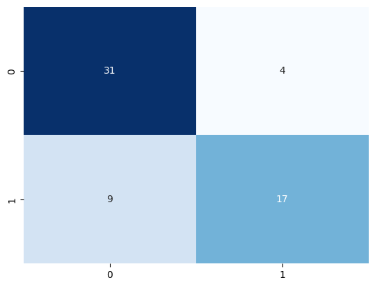
Let’s examine the model’s confusion matrix and accuracy to assess its performance.

# Create confusion matrix
cm = confusion_matrix(y_test, y_pred.round())

# Visualize confusion matrix using seaborn heatmap
sns.heatmap(cm, annot=True, cmap="Blues", fmt="d", cbar=False)

# Calculate and print accuracy score
ac = accuracy_score(y_test, y_pred.round())
print('accuracy of the model: ', ac)

accuracy of the model:  0.7868852459016393

22.4. Your turn! 🚀#

Try the exercises about neural networks classify 15 fruits and neural networks for classification.

HIGHLY RECOMMENDED LECTURE : The spelled-out intro to neural networks and backpropagation: building micrograd by Andrej Karpathy It only assumes basic knowledge of Python and a vague recollection of calculus from high school. Github Repo

22.5. Acknowledgments#

Thanks to Pragati Baheti and Rajesh kumar jha for creating the open-source course The Essential Guide to Neural Network Architectures and Heart Disease Classification - Neural Network, as well as Andrej Karpathy for sharing his brillant thoughts. It inspires the majority of the content in this chapter.

Ocademy Open Machine Learning Book

Neural Networks

Contents