42.106. Intro to Autoencoders#

This tutorial introduces autoencoders with three examples: the basics, image denoising, and anomaly detection.

An autoencoder is a special type of neural network that is trained to copy its input to its output. For example, given an image of a handwritten digit, an autoencoder first encodes the image into a lower dimensional latent representation, then decodes the latent representation back to an image. An autoencoder learns to compress the data while minimizing the reconstruction error.

To learn more about autoencoders, please consider reading chapter 14 from Deep Learning by Ian Goodfellow, Yoshua Bengio, and Aaron Courville.

42.106.1. Import TensorFlow and other libraries#

import matplotlib.pyplot as plt
import numpy as np
import pandas as pd
import tensorflow as tf

from sklearn.metrics import accuracy_score, precision_score, recall_score
from sklearn.model_selection import train_test_split
from tensorflow.keras import layers, losses
from tensorflow.keras.datasets import fashion_mnist
from tensorflow.keras.models import Model

42.106.2. Download models#

import os
import requests
import zipfile

basic_autoencoder_model_url = "https://static-1300131294.cos.ap-shanghai.myqcloud.com/data/deep-learning/autoencoder/autoencoder/basic_autoencoder_model.zip"
convolutional_autoencoder_model_url = "https://static-1300131294.cos.ap-shanghai.myqcloud.com/data/deep-learning/autoencoder/autoencoder/convolutional_autoencoder_model.zip"
ecg_autoencoder_model_url = "https://static-1300131294.cos.ap-shanghai.myqcloud.com/data/deep-learning/autoencoder/autoencoder/ecg_autoencoder_model.zip"

notebook_path = os.getcwd()

tmp_folder_path = os.path.join(notebook_path, "tmp")

if not os.path.exists(tmp_folder_path):
    os.makedirs(tmp_folder_path)

file_path = os.path.join(tmp_folder_path,"autoencoder")

if not os.path.exists(file_path):
    os.makedirs(file_path)

zip_store_path = os.path.join(file_path, "zip-store")

if not os.path.exists(zip_store_path):
    os.makedirs(zip_store_path)

basic_autoencoder_model_response = requests.get(basic_autoencoder_model_url)
convolutional_autoencoder_model_response = requests.get(convolutional_autoencoder_model_url)
ecg_autoencoder_model_response = requests.get(ecg_autoencoder_model_url)

basic_autoencoder_model_name = os.path.basename(basic_autoencoder_model_url)
convolutional_autoencoder_model_name = os.path.basename(convolutional_autoencoder_model_url)
ecg_autoencoder_model_name = os.path.basename(ecg_autoencoder_model_url)

basic_autoencoder_model_save_path = os.path.join(zip_store_path, basic_autoencoder_model_name)
convolutional_autoencoder_model_save_path = os.path.join(zip_store_path, convolutional_autoencoder_model_name)
ecg_autoencoder_model_save_path = os.path.join(zip_store_path, ecg_autoencoder_model_name)

with open(basic_autoencoder_model_save_path, "wb") as file:
    file.write(basic_autoencoder_model_response.content)
    
with open(convolutional_autoencoder_model_save_path, "wb") as file:
    file.write(convolutional_autoencoder_model_response.content)

with open(ecg_autoencoder_model_save_path, "wb") as file:
    file.write(ecg_autoencoder_model_response.content)

bam_zip_file_path = f"./tmp/autoencoder/zip-store/{basic_autoencoder_model_name}"
bam_extract_path = "./tmp/autoencoder/basic_autoencoder_model"

cam_zip_file_path = f"./tmp/autoencoder/zip-store/{convolutional_autoencoder_model_name}"
cam_extract_path = "./tmp/autoencoder/convolutional_autoencoder_model"

ecg_zip_file_path = f"./tmp/autoencoder/zip-store/{ecg_autoencoder_model_name}"
ecg_extract_path = "./tmp/autoencoder/ecg_autoencoder_model"

zip_ref = zipfile.ZipFile(bam_zip_file_path, 'r')
zip_ref.extractall(bam_extract_path)
zip_ref.close()

zip_ref = zipfile.ZipFile(cam_zip_file_path, 'r')
zip_ref.extractall(cam_extract_path)
zip_ref.close()

zip_ref = zipfile.ZipFile(ecg_zip_file_path, 'r')
zip_ref.extractall(ecg_extract_path)
zip_ref.close()

42.106.3. Load the dataset#

To start, you will train the basic autoencoder using the Fashion MNIST dataset. Each image in this dataset is 28x28 pixels.

(x_train, _), (x_test, _) = fashion_mnist.load_data()

x_train = x_train.astype('float32') / 255.
x_test = x_test.astype('float32') / 255.

print (x_train.shape)
print (x_test.shape)

(60000, 28, 28)
(10000, 28, 28)

42.106.4. First example: Basic autoencoder#

Basic autoencoder results

Define an autoencoder with two Dense layers: an encoder, which compresses the images into a 64 dimensional latent vector, and a decoder, that reconstructs the original image from the latent space.

To define your model, use the Keras Model Subclassing API.

latent_dim = 64 

class Autoencoder(Model):
  def __init__(self, latent_dim):
    super(Autoencoder, self).__init__()
    self.latent_dim = latent_dim   
    self.encoder = tf.keras.Sequential([
      layers.Flatten(),
      layers.Dense(latent_dim, activation='relu'),
    ])
    self.decoder = tf.keras.Sequential([
      layers.Dense(784, activation='sigmoid'),
      layers.Reshape((28, 28))
    ])

  def call(self, x):
    encoded = self.encoder(x)
    decoded = self.decoder(encoded)
    return decoded
  
autoencoder = Autoencoder(latent_dim) 

autoencoder.compile(optimizer='adam', loss=losses.MeanSquaredError())

Train the model using x_train as both the input and the target. The encoder will learn to compress the dataset from 784 dimensions to the latent space, and the decoder will learn to reconstruct the original images.

# autoencoder.fit(x_train, x_train,
#                 epochs=10,
#                 shuffle=True,
#                 validation_data=(x_test, x_test))
# autoencoder.save('basic_autoencoder_model', save_format='tf')

To save time, just load the model.

autoencoder = tf.keras.models.load_model('./tmp/autoencoder/basic_autoencoder_model')

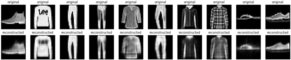
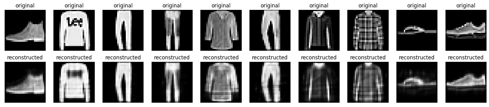
Now that the model is trained, let’s test it by encoding and decoding images from the test set.

encoded_imgs = autoencoder.encoder(x_test).numpy()
decoded_imgs = autoencoder.decoder(encoded_imgs).numpy()

n = 10
plt.figure(figsize=(20, 4))
for i in range(n):
  # display original
  ax = plt.subplot(2, n, i + 1)
  plt.imshow(x_test[i])
  plt.title("original")
  plt.gray()
  ax.get_xaxis().set_visible(False)
  ax.get_yaxis().set_visible(False)

  # display reconstruction
  ax = plt.subplot(2, n, i + 1 + n)
  plt.imshow(decoded_imgs[i])
  plt.title("reconstructed")
  plt.gray()
  ax.get_xaxis().set_visible(False)
  ax.get_yaxis().set_visible(False)
plt.show()

42.106.5. Second example: Image denoising#

Image denoising results

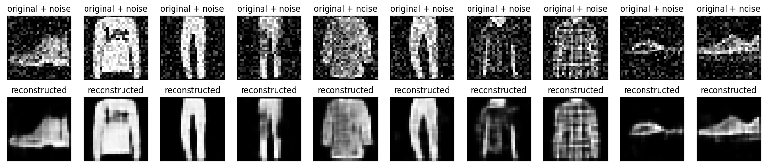
An autoencoder can also be trained to remove noise from images. In the following section, you will create a noisy version of the Fashion MNIST dataset by applying random noise to each image. You will then train an autoencoder using the noisy image as input, and the original image as the target.

Let’s reimport the dataset to omit the modifications made earlier.

(x_train, _), (x_test, _) = fashion_mnist.load_data()

x_train = x_train.astype('float32') / 255.
x_test = x_test.astype('float32') / 255.

x_train = x_train[..., tf.newaxis]
x_test = x_test[..., tf.newaxis]

print(x_train.shape)

(60000, 28, 28, 1)

Adding random noise to the images

noise_factor = 0.2
x_train_noisy = x_train + noise_factor * tf.random.normal(shape=x_train.shape) 
x_test_noisy = x_test + noise_factor * tf.random.normal(shape=x_test.shape) 

x_train_noisy = tf.clip_by_value(x_train_noisy, clip_value_min=0., clip_value_max=1.)
x_test_noisy = tf.clip_by_value(x_test_noisy, clip_value_min=0., clip_value_max=1.)

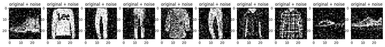
Plot the noisy images.

n = 10
plt.figure(figsize=(20, 2))
for i in range(n):
    ax = plt.subplot(1, n, i + 1)
    plt.title("original + noise")
    plt.imshow(tf.squeeze(x_test_noisy[i]))
    plt.gray()
plt.show()

42.106.5.1. Define a convolutional autoencoder#

In this example, you will train a convolutional autoencoder using Conv2D layers in the encoder, and Conv2DTranspose layers in the decoder.

class Denoise(Model):
  def __init__(self):
    super(Denoise, self).__init__()
    self.encoder = tf.keras.Sequential([
      layers.Input(shape=(28, 28, 1)),
      layers.Conv2D(16, (3, 3), activation='relu', padding='same', strides=2),
      layers.Conv2D(8, (3, 3), activation='relu', padding='same', strides=2)])

    self.decoder = tf.keras.Sequential([
      layers.Conv2DTranspose(8, kernel_size=3, strides=2, activation='relu', padding='same'),
      layers.Conv2DTranspose(16, kernel_size=3, strides=2, activation='relu', padding='same'),
      layers.Conv2D(1, kernel_size=(3, 3), activation='sigmoid', padding='same')])

  def call(self, x):
    encoded = self.encoder(x)
    decoded = self.decoder(encoded)
    return decoded

autoencoder = Denoise()

autoencoder.compile(optimizer='adam', loss=losses.MeanSquaredError())

# autoencoder.fit(x_train_noisy, x_train,
#                 epochs=10,
#                 shuffle=True,
#                 validation_data=(x_test_noisy, x_test))

# autoencoder.save('convolutional_autoencoder_model', save_format='tf')

autoencoder = tf.keras.models.load_model('./tmp/autoencoder/convolutional_autoencoder_model')

Let’s take a look at a summary of the encoder. Notice how the images are downsampled from 28x28 to 7x7.

autoencoder.encoder.summary()

Model: "sequential_2"
_________________________________________________________________
 Layer (type)                Output Shape              Param #   
=================================================================
 conv2d (Conv2D)             (None, 14, 14, 16)        160       
                                                                 
 conv2d_1 (Conv2D)           (None, 7, 7, 8)           1160      
                                                                 
=================================================================
Total params: 1320 (5.16 KB)
Trainable params: 1320 (5.16 KB)
Non-trainable params: 0 (0.00 Byte)
_________________________________________________________________

The decoder upsamples the images back from 7x7 to 28x28.

autoencoder.decoder.summary()

Model: "sequential_3"
_________________________________________________________________
 Layer (type)                Output Shape              Param #   
=================================================================
 conv2d_transpose (Conv2DTr  (None, 14, 14, 8)         584       
 anspose)                                                        
                                                                 
 conv2d_transpose_1 (Conv2D  (None, 28, 28, 16)        1168      
 Transpose)                                                      
                                                                 
 conv2d_2 (Conv2D)           (None, 28, 28, 1)         145       
                                                                 
=================================================================
Total params: 1897 (7.41 KB)
Trainable params: 1897 (7.41 KB)
Non-trainable params: 0 (0.00 Byte)
_________________________________________________________________

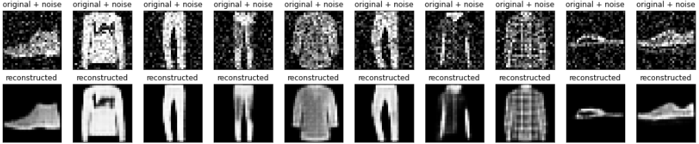
Plotting both the noisy images and the denoised images produced by the autoencoder.

encoded_imgs = autoencoder.encoder(x_test_noisy).numpy()
decoded_imgs = autoencoder.decoder(encoded_imgs).numpy()

n = 10
plt.figure(figsize=(20, 4))
for i in range(n):

    # display original + noise
    ax = plt.subplot(2, n, i + 1)
    plt.title("original + noise")
    plt.imshow(tf.squeeze(x_test_noisy[i]))
    plt.gray()
    ax.get_xaxis().set_visible(False)
    ax.get_yaxis().set_visible(False)

    # display reconstruction
    bx = plt.subplot(2, n, i + n + 1)
    plt.title("reconstructed")
    plt.imshow(tf.squeeze(decoded_imgs[i]))
    plt.gray()
    bx.get_xaxis().set_visible(False)
    bx.get_yaxis().set_visible(False)
plt.show()

42.106.6. Third example: Anomaly detection#

42.106.7. Overview#

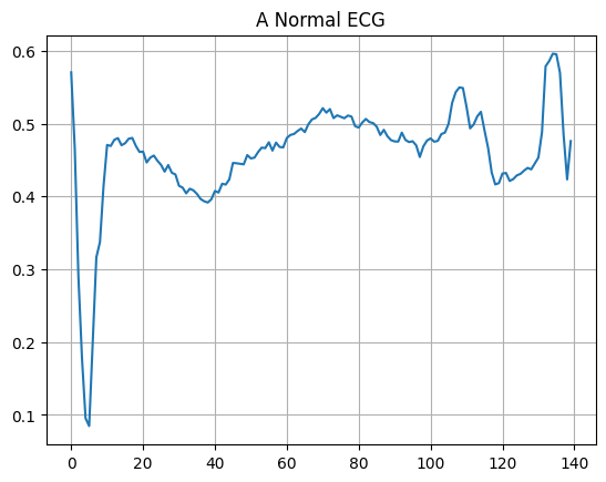
In this example, you will train an autoencoder to detect anomalies on the ECG5000 dataset. This dataset contains 5,000 Electrocardiograms, each with 140 data points. You will use a simplified version of the dataset, where each example has been labeled either 0 (corresponding to an abnormal rhythm), or 1 (corresponding to a normal rhythm). You are interested in identifying the abnormal rhythms.

Note: This is a labeled dataset, so you could phrase this as a supervised learning problem. The goal of this example is to illustrate anomaly detection concepts you can apply to larger datasets, where you do not have labels available (for example, if you had many thousands of normal rhythms, and only a small number of abnormal rhythms).

How will you detect anomalies using an autoencoder? Recall that an autoencoder is trained to minimize reconstruction error. You will train an autoencoder on the normal rhythms only, then use it to reconstruct all the data. Our hypothesis is that the abnormal rhythms will have higher reconstruction error. You will then classify a rhythm as an anomaly if the reconstruction error surpasses a fixed threshold.

42.106.7.1. Load ECG data#

The dataset you will use is based on one from timeseriesclassification.com.

datasets_url = "https://static-1300131294.cos.ap-shanghai.myqcloud.com/data/deep-learning/autoencoder/autoencoder/autoencoder_ecg.zip"

notebook_path = os.getcwd()

tmp_folder_path = os.path.join(notebook_path, "tmp")

if not os.path.exists(tmp_folder_path):
    os.makedirs(tmp_folder_path)
    
file_path = os.path.join(tmp_folder_path,"autoencoder")

if not os.path.exists(file_path):
    os.makedirs(file_path)

zip_store_path = os.path.join(file_path, "zip-store")

if not os.path.exists(zip_store_path):
    os.makedirs(zip_store_path)
    
datasets_response = requests.get(datasets_url)

datasets_name = os.path.basename(datasets_url)

datasets_save_path = os.path.join(zip_store_path, datasets_name)

with open(datasets_save_path, "wb") as file:
    file.write(datasets_response.content)

zip_file_path = f"./tmp/autoencoder/zip-store/{datasets_name}"
extract_path = "./tmp/autoencoder"

zip_ref = zipfile.ZipFile(zip_file_path, 'r')
zip_ref.extractall(extract_path)
zip_ref.close()

dataframe = pd.read_csv("./tmp/autoencoder/autoencoder_ecg.csv", header=None)
raw_data = dataframe.values
dataframe.head()

	0	1	2	3	4	5	6	7	8	9	...	131	132	133	134	135	136	137	138	139	140
0	-0.112522	-2.827204	-3.773897	-4.349751	-4.376041	-3.474986	-2.181408	-1.818286	-1.250522	-0.477492	...	0.792168	0.933541	0.796958	0.578621	0.257740	0.228077	0.123431	0.925286	0.193137	1.0
1	-1.100878	-3.996840	-4.285843	-4.506579	-4.022377	-3.234368	-1.566126	-0.992258	-0.754680	0.042321	...	0.538356	0.656881	0.787490	0.724046	0.555784	0.476333	0.773820	1.119621	-1.436250	1.0
2	-0.567088	-2.593450	-3.874230	-4.584095	-4.187449	-3.151462	-1.742940	-1.490659	-1.183580	-0.394229	...	0.886073	0.531452	0.311377	-0.021919	-0.713683	-0.532197	0.321097	0.904227	-0.421797	1.0
3	0.490473	-1.914407	-3.616364	-4.318823	-4.268016	-3.881110	-2.993280	-1.671131	-1.333884	-0.965629	...	0.350816	0.499111	0.600345	0.842069	0.952074	0.990133	1.086798	1.403011	-0.383564	1.0
4	0.800232	-0.874252	-2.384761	-3.973292	-4.338224	-3.802422	-2.534510	-1.783423	-1.594450	-0.753199	...	1.148884	0.958434	1.059025	1.371682	1.277392	0.960304	0.971020	1.614392	1.421456	1.0

5 rows × 141 columns

# The last element contains the labels
labels = raw_data[:, -1]

# The other data points are the electrocadriogram data
data = raw_data[:, 0:-1]

train_data, test_data, train_labels, test_labels = train_test_split(
    data, labels, test_size=0.2, random_state=21
)

Normalize the data to [0,1].

min_val = tf.reduce_min(train_data)
max_val = tf.reduce_max(train_data)

train_data = (train_data - min_val) / (max_val - min_val)
test_data = (test_data - min_val) / (max_val - min_val)

train_data = tf.cast(train_data, tf.float32)
test_data = tf.cast(test_data, tf.float32)

You will train the autoencoder using only the normal rhythms, which are labeled in this dataset as 1. Separate the normal rhythms from the abnormal rhythms.

train_labels = train_labels.astype(bool)
test_labels = test_labels.astype(bool)

normal_train_data = train_data[train_labels]
normal_test_data = test_data[test_labels]

anomalous_train_data = train_data[~train_labels]
anomalous_test_data = test_data[~test_labels]

Plot a normal ECG.

plt.grid()
plt.plot(np.arange(140), normal_train_data[0])
plt.title("A Normal ECG")
plt.show()

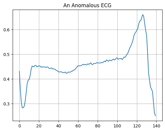
Plot an anomalous ECG.

plt.grid()
plt.plot(np.arange(140), anomalous_train_data[0])
plt.title("An Anomalous ECG")
plt.show()

42.106.7.2. Build the model#

class AnomalyDetector(Model):
  def __init__(self):
    super(AnomalyDetector, self).__init__()
    self.encoder = tf.keras.Sequential([
      layers.Dense(32, activation="relu"),
      layers.Dense(16, activation="relu"),
      layers.Dense(8, activation="relu")])
    
    self.decoder = tf.keras.Sequential([
      layers.Dense(16, activation="relu"),
      layers.Dense(32, activation="relu"),
      layers.Dense(140, activation="sigmoid")])
    
  def call(self, x):
    encoded = self.encoder(x)
    decoded = self.decoder(encoded)
    return decoded

autoencoder = AnomalyDetector()

autoencoder.compile(optimizer='adam', loss='mae')

Notice that the autoencoder is trained using only the normal ECGs, but is evaluated using the full test set.

# history = autoencoder.fit(normal_train_data, normal_train_data, 
#           epochs=20, 
#           batch_size=512,
#           validation_data=(test_data, test_data),
#           shuffle=True)

# autoencoder.save('ecg_autoencoder_model', save_format='tf')

autoencoder = tf.keras.models.load_model('./tmp/autoencoder/ecg_autoencoder_model')

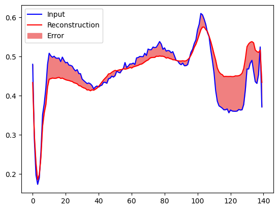
You will soon classify an ECG as anomalous if the reconstruction error is greater than one standard deviation from the normal training examples. First, let’s plot a normal ECG from the training set, the reconstruction after it’s encoded and decoded by the autoencoder, and the reconstruction error.

encoded_data = autoencoder.encoder(normal_test_data).numpy()
decoded_data = autoencoder.decoder(encoded_data).numpy()

plt.plot(normal_test_data[0], 'b')
plt.plot(decoded_data[0], 'r')
plt.fill_between(np.arange(140), decoded_data[0], normal_test_data[0], color='lightcoral')
plt.legend(labels=["Input", "Reconstruction", "Error"])
plt.show()

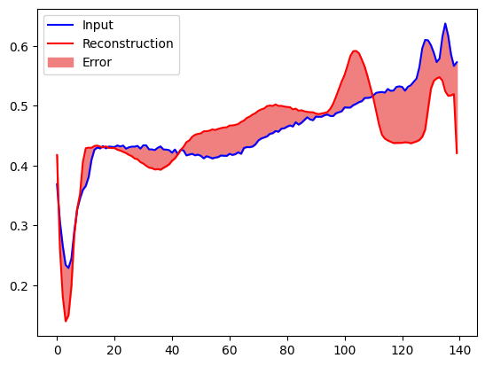
Create a similar plot, this time for an anomalous test example.

encoded_data = autoencoder.encoder(anomalous_test_data).numpy()
decoded_data = autoencoder.decoder(encoded_data).numpy()

plt.plot(anomalous_test_data[0], 'b')
plt.plot(decoded_data[0], 'r')
plt.fill_between(np.arange(140), decoded_data[0], anomalous_test_data[0], color='lightcoral')
plt.legend(labels=["Input", "Reconstruction", "Error"])
plt.show()

42.106.7.3. Detect anomalies#

Detect anomalies by calculating whether the reconstruction loss is greater than a fixed threshold. In this tutorial, you will calculate the mean average error for normal examples from the training set, then classify future examples as anomalous if the reconstruction error is higher than one standard deviation from the training set.

Plot the reconstruction error on normal ECGs from the training set

reconstructions = autoencoder.predict(normal_train_data)
train_loss = tf.keras.losses.mae(reconstructions, normal_train_data)

plt.hist(train_loss[None,:], bins=50)
plt.xlabel("Train loss")
plt.ylabel("No of examples")
plt.show()

74/74 [==============================] - 1s 4ms/step

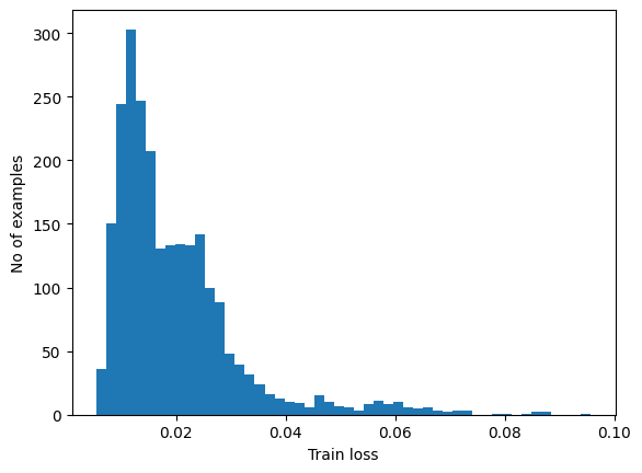
Choose a threshold value that is one standard deviations above the mean.

threshold = np.mean(train_loss) + np.std(train_loss)
print("Threshold: ", threshold)

Threshold:  0.031506725

Note: There are other strategies you could use to select a threshold value above which test examples should be classified as anomalous, the correct approach will depend on your dataset. You can learn more with the links at the end of this tutorial.

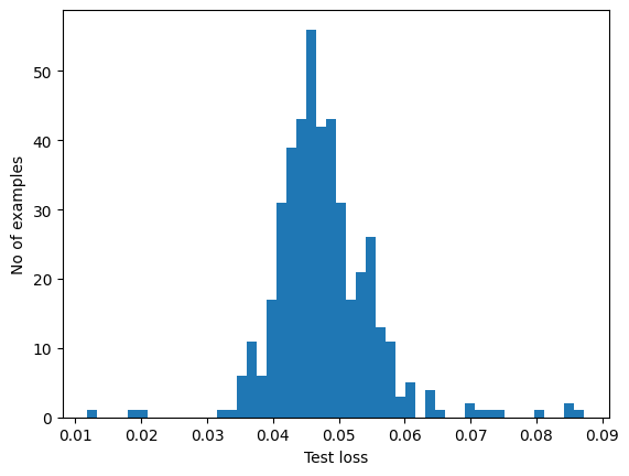
If you examine the reconstruction error for the anomalous examples in the test set, you’ll notice most have greater reconstruction error than the threshold. By varing the threshold, you can adjust the precision and recall of your classifier.

reconstructions = autoencoder.predict(anomalous_test_data)
test_loss = tf.keras.losses.mae(reconstructions, anomalous_test_data)

plt.hist(test_loss[None, :], bins=50)
plt.xlabel("Test loss")
plt.ylabel("No of examples")
plt.show()

14/14 [==============================] - 0s 3ms/step

Classify an ECG as an anomaly if the reconstruction error is greater than the threshold.

def predict(model, data, threshold):
  reconstructions = model(data)
  loss = tf.keras.losses.mae(reconstructions, data)
  return tf.math.less(loss, threshold)

def print_stats(predictions, labels):
  print("Accuracy = {}".format(accuracy_score(labels, predictions)))
  print("Precision = {}".format(precision_score(labels, predictions)))
  print("Recall = {}".format(recall_score(labels, predictions)))

preds = predict(autoencoder, test_data, threshold)
print_stats(preds, test_labels)

Accuracy = 0.94
Precision = 0.9940711462450593
Recall = 0.8982142857142857

42.106.8. Next steps#

To learn more about anomaly detection with autoencoders, check out this excellent interactive example built with TensorFlow.js by Victor Dibia. For a real-world use case, you can learn how Airbus Detects Anomalies in ISS Telemetry Data using TensorFlow. To learn more about the basics, consider reading this blog post by François Chollet. For more details, check out chapter 14 from Deep Learning by Ian Goodfellow, Yoshua Bengio, and Aaron Courville.

42.106.9. Acknowledgments#

Thanks to TensorFlow Core for creating the open-source course autoencoder. It inspires the majority of the content in this chapter.

Ocademy Open Machine Learning Book

Intro to Autoencoders

Contents