Machine Learning overview - assignment 1
Contents
42.42. Machine Learning overview - assignment 1#
42.42.1. What the assignment is for#
In this assignment, we will explore the very classic iris dataset and use the very simple KNN (K-Nearest Neighbors) algorithm for classification.
You should pay attention to how this assignment follows the Machine Learning Workflow in our lecture session!
42.42.2. Import libraries#
%matplotlib inline
import pandas
import numpy
from matplotlib import pyplot as plt
42.42.3. Load Dataset#
NOTE: Iris dataset includes three iris species with 50 samples each as well as some properties about each flower. One flower species is linearly separable from the other two, but the other two are not linearly separable from each other.
iris = pandas.read_csv(
    "https://static-1300131294.cos.ap-shanghai.myqcloud.com/data/data-science/working-with-data/pandas/iris.csv"
)
42.42.4. Dimension (shape) of Dataset#
We can get a quick idea of how many instances (rows) and how many attributes (columns) the data contains with the shape property.
print(iris.shape)
(150, 5)
42.42.5. Show the first 5 rows of the data#
print(iris.head(5))
   SepalLength  SepalWidth  PetalLength  PetalWidth         Name
0          5.1         3.5          1.4         0.2  Iris-setosa
1          4.9         3.0          1.4         0.2  Iris-setosa
2          4.7         3.2          1.3         0.2  Iris-setosa
3          4.6         3.1          1.5         0.2  Iris-setosa
4          5.0         3.6          1.4         0.2  Iris-setosa
42.42.6. Get a global description of the dataset#
print(iris.describe())
       SepalLength  SepalWidth  PetalLength  PetalWidth
count   150.000000  150.000000   150.000000  150.000000
mean      5.843333    3.054000     3.758667    1.198667
std       0.828066    0.433594     1.764420    0.763161
min       4.300000    2.000000     1.000000    0.100000
25%       5.100000    2.800000     1.600000    0.300000
50%       5.800000    3.000000     4.350000    1.300000
75%       6.400000    3.300000     5.100000    1.800000
max       7.900000    4.400000     6.900000    2.500000
42.42.7. Group data#
Let’s now take a look at the number of instances (rows) that belong to each class. We can view this as an absolute count.
print(iris.groupby("Name").size())
Name
Iris-setosa        50
Iris-versicolor    50
Iris-virginica     50
dtype: int64
42.42.8. Dividing data into features and labels#
As we can see dataset contain five columns: SepalLength, SepalWidth, PetalLength, PetalWidth and Name. The actual features are described by columns 0-3. Last column contains labels of samples. Firstly we need to split data into two arrays: X (features) and y (labels).
feature_columns = ["SepalLength", "SepalWidth", "PetalLength", "PetalWidth"]
X = iris[feature_columns].values
y = iris["Name"].values
X
array([[5.1, 3.5, 1.4, 0.2],
       [4.9, 3. , 1.4, 0.2],
       [4.7, 3.2, 1.3, 0.2],
       [4.6, 3.1, 1.5, 0.2],
       [5. , 3.6, 1.4, 0.2],
       [5.4, 3.9, 1.7, 0.4],
       [4.6, 3.4, 1.4, 0.3],
       [5. , 3.4, 1.5, 0.2],
       [4.4, 2.9, 1.4, 0.2],
       [4.9, 3.1, 1.5, 0.1],
       [5.4, 3.7, 1.5, 0.2],
       [4.8, 3.4, 1.6, 0.2],
       [4.8, 3. , 1.4, 0.1],
       [4.3, 3. , 1.1, 0.1],
       [5.8, 4. , 1.2, 0.2],
       [5.7, 4.4, 1.5, 0.4],
       [5.4, 3.9, 1.3, 0.4],
       [5.1, 3.5, 1.4, 0.3],
       [5.7, 3.8, 1.7, 0.3],
       [5.1, 3.8, 1.5, 0.3],
       [5.4, 3.4, 1.7, 0.2],
       [5.1, 3.7, 1.5, 0.4],
       [4.6, 3.6, 1. , 0.2],
       [5.1, 3.3, 1.7, 0.5],
       [4.8, 3.4, 1.9, 0.2],
       [5. , 3. , 1.6, 0.2],
       [5. , 3.4, 1.6, 0.4],
       [5.2, 3.5, 1.5, 0.2],
       [5.2, 3.4, 1.4, 0.2],
       [4.7, 3.2, 1.6, 0.2],
       [4.8, 3.1, 1.6, 0.2],
       [5.4, 3.4, 1.5, 0.4],
       [5.2, 4.1, 1.5, 0.1],
       [5.5, 4.2, 1.4, 0.2],
       [4.9, 3.1, 1.5, 0.1],
       [5. , 3.2, 1.2, 0.2],
       [5.5, 3.5, 1.3, 0.2],
       [4.9, 3.1, 1.5, 0.1],
       [4.4, 3. , 1.3, 0.2],
       [5.1, 3.4, 1.5, 0.2],
       [5. , 3.5, 1.3, 0.3],
       [4.5, 2.3, 1.3, 0.3],
       [4.4, 3.2, 1.3, 0.2],
       [5. , 3.5, 1.6, 0.6],
       [5.1, 3.8, 1.9, 0.4],
       [4.8, 3. , 1.4, 0.3],
       [5.1, 3.8, 1.6, 0.2],
       [4.6, 3.2, 1.4, 0.2],
       [5.3, 3.7, 1.5, 0.2],
       [5. , 3.3, 1.4, 0.2],
       [7. , 3.2, 4.7, 1.4],
       [6.4, 3.2, 4.5, 1.5],
       [6.9, 3.1, 4.9, 1.5],
       [5.5, 2.3, 4. , 1.3],
       [6.5, 2.8, 4.6, 1.5],
       [5.7, 2.8, 4.5, 1.3],
       [6.3, 3.3, 4.7, 1.6],
       [4.9, 2.4, 3.3, 1. ],
       [6.6, 2.9, 4.6, 1.3],
       [5.2, 2.7, 3.9, 1.4],
       [5. , 2. , 3.5, 1. ],
       [5.9, 3. , 4.2, 1.5],
       [6. , 2.2, 4. , 1. ],
       [6.1, 2.9, 4.7, 1.4],
       [5.6, 2.9, 3.6, 1.3],
       [6.7, 3.1, 4.4, 1.4],
       [5.6, 3. , 4.5, 1.5],
       [5.8, 2.7, 4.1, 1. ],
       [6.2, 2.2, 4.5, 1.5],
       [5.6, 2.5, 3.9, 1.1],
       [5.9, 3.2, 4.8, 1.8],
       [6.1, 2.8, 4. , 1.3],
       [6.3, 2.5, 4.9, 1.5],
       [6.1, 2.8, 4.7, 1.2],
       [6.4, 2.9, 4.3, 1.3],
       [6.6, 3. , 4.4, 1.4],
       [6.8, 2.8, 4.8, 1.4],
       [6.7, 3. , 5. , 1.7],
       [6. , 2.9, 4.5, 1.5],
       [5.7, 2.6, 3.5, 1. ],
       [5.5, 2.4, 3.8, 1.1],
       [5.5, 2.4, 3.7, 1. ],
       [5.8, 2.7, 3.9, 1.2],
       [6. , 2.7, 5.1, 1.6],
       [5.4, 3. , 4.5, 1.5],
       [6. , 3.4, 4.5, 1.6],
       [6.7, 3.1, 4.7, 1.5],
       [6.3, 2.3, 4.4, 1.3],
       [5.6, 3. , 4.1, 1.3],
       [5.5, 2.5, 4. , 1.3],
       [5.5, 2.6, 4.4, 1.2],
       [6.1, 3. , 4.6, 1.4],
       [5.8, 2.6, 4. , 1.2],
       [5. , 2.3, 3.3, 1. ],
       [5.6, 2.7, 4.2, 1.3],
       [5.7, 3. , 4.2, 1.2],
       [5.7, 2.9, 4.2, 1.3],
       [6.2, 2.9, 4.3, 1.3],
       [5.1, 2.5, 3. , 1.1],
       [5.7, 2.8, 4.1, 1.3],
       [6.3, 3.3, 6. , 2.5],
       [5.8, 2.7, 5.1, 1.9],
       [7.1, 3. , 5.9, 2.1],
       [6.3, 2.9, 5.6, 1.8],
       [6.5, 3. , 5.8, 2.2],
       [7.6, 3. , 6.6, 2.1],
       [4.9, 2.5, 4.5, 1.7],
       [7.3, 2.9, 6.3, 1.8],
       [6.7, 2.5, 5.8, 1.8],
       [7.2, 3.6, 6.1, 2.5],
       [6.5, 3.2, 5.1, 2. ],
       [6.4, 2.7, 5.3, 1.9],
       [6.8, 3. , 5.5, 2.1],
       [5.7, 2.5, 5. , 2. ],
       [5.8, 2.8, 5.1, 2.4],
       [6.4, 3.2, 5.3, 2.3],
       [6.5, 3. , 5.5, 1.8],
       [7.7, 3.8, 6.7, 2.2],
       [7.7, 2.6, 6.9, 2.3],
       [6. , 2.2, 5. , 1.5],
       [6.9, 3.2, 5.7, 2.3],
       [5.6, 2.8, 4.9, 2. ],
       [7.7, 2.8, 6.7, 2. ],
       [6.3, 2.7, 4.9, 1.8],
       [6.7, 3.3, 5.7, 2.1],
       [7.2, 3.2, 6. , 1.8],
       [6.2, 2.8, 4.8, 1.8],
       [6.1, 3. , 4.9, 1.8],
       [6.4, 2.8, 5.6, 2.1],
       [7.2, 3. , 5.8, 1.6],
       [7.4, 2.8, 6.1, 1.9],
       [7.9, 3.8, 6.4, 2. ],
       [6.4, 2.8, 5.6, 2.2],
       [6.3, 2.8, 5.1, 1.5],
       [6.1, 2.6, 5.6, 1.4],
       [7.7, 3. , 6.1, 2.3],
       [6.3, 3.4, 5.6, 2.4],
       [6.4, 3.1, 5.5, 1.8],
       [6. , 3. , 4.8, 1.8],
       [6.9, 3.1, 5.4, 2.1],
       [6.7, 3.1, 5.6, 2.4],
       [6.9, 3.1, 5.1, 2.3],
       [5.8, 2.7, 5.1, 1.9],
       [6.8, 3.2, 5.9, 2.3],
       [6.7, 3.3, 5.7, 2.5],
       [6.7, 3. , 5.2, 2.3],
       [6.3, 2.5, 5. , 1.9],
       [6.5, 3. , 5.2, 2. ],
       [6.2, 3.4, 5.4, 2.3],
       [5.9, 3. , 5.1, 1.8]])
y
array(['Iris-setosa', 'Iris-setosa', 'Iris-setosa', 'Iris-setosa',
       'Iris-setosa', 'Iris-setosa', 'Iris-setosa', 'Iris-setosa',
       'Iris-setosa', 'Iris-setosa', 'Iris-setosa', 'Iris-setosa',
       'Iris-setosa', 'Iris-setosa', 'Iris-setosa', 'Iris-setosa',
       'Iris-setosa', 'Iris-setosa', 'Iris-setosa', 'Iris-setosa',
       'Iris-setosa', 'Iris-setosa', 'Iris-setosa', 'Iris-setosa',
       'Iris-setosa', 'Iris-setosa', 'Iris-setosa', 'Iris-setosa',
       'Iris-setosa', 'Iris-setosa', 'Iris-setosa', 'Iris-setosa',
       'Iris-setosa', 'Iris-setosa', 'Iris-setosa', 'Iris-setosa',
       'Iris-setosa', 'Iris-setosa', 'Iris-setosa', 'Iris-setosa',
       'Iris-setosa', 'Iris-setosa', 'Iris-setosa', 'Iris-setosa',
       'Iris-setosa', 'Iris-setosa', 'Iris-setosa', 'Iris-setosa',
       'Iris-setosa', 'Iris-setosa', 'Iris-versicolor', 'Iris-versicolor',
       'Iris-versicolor', 'Iris-versicolor', 'Iris-versicolor',
       'Iris-versicolor', 'Iris-versicolor', 'Iris-versicolor',
       'Iris-versicolor', 'Iris-versicolor', 'Iris-versicolor',
       'Iris-versicolor', 'Iris-versicolor', 'Iris-versicolor',
       'Iris-versicolor', 'Iris-versicolor', 'Iris-versicolor',
       'Iris-versicolor', 'Iris-versicolor', 'Iris-versicolor',
       'Iris-versicolor', 'Iris-versicolor', 'Iris-versicolor',
       'Iris-versicolor', 'Iris-versicolor', 'Iris-versicolor',
       'Iris-versicolor', 'Iris-versicolor', 'Iris-versicolor',
       'Iris-versicolor', 'Iris-versicolor', 'Iris-versicolor',
       'Iris-versicolor', 'Iris-versicolor', 'Iris-versicolor',
       'Iris-versicolor', 'Iris-versicolor', 'Iris-versicolor',
       'Iris-versicolor', 'Iris-versicolor', 'Iris-versicolor',
       'Iris-versicolor', 'Iris-versicolor', 'Iris-versicolor',
       'Iris-versicolor', 'Iris-versicolor', 'Iris-versicolor',
       'Iris-versicolor', 'Iris-versicolor', 'Iris-versicolor',
       'Iris-virginica', 'Iris-virginica', 'Iris-virginica',
       'Iris-virginica', 'Iris-virginica', 'Iris-virginica',
       'Iris-virginica', 'Iris-virginica', 'Iris-virginica',
       'Iris-virginica', 'Iris-virginica', 'Iris-virginica',
       'Iris-virginica', 'Iris-virginica', 'Iris-virginica',
       'Iris-virginica', 'Iris-virginica', 'Iris-virginica',
       'Iris-virginica', 'Iris-virginica', 'Iris-virginica',
       'Iris-virginica', 'Iris-virginica', 'Iris-virginica',
       'Iris-virginica', 'Iris-virginica', 'Iris-virginica',
       'Iris-virginica', 'Iris-virginica', 'Iris-virginica',
       'Iris-virginica', 'Iris-virginica', 'Iris-virginica',
       'Iris-virginica', 'Iris-virginica', 'Iris-virginica',
       'Iris-virginica', 'Iris-virginica', 'Iris-virginica',
       'Iris-virginica', 'Iris-virginica', 'Iris-virginica',
       'Iris-virginica', 'Iris-virginica', 'Iris-virginica',
       'Iris-virginica', 'Iris-virginica', 'Iris-virginica',
       'Iris-virginica', 'Iris-virginica'], dtype=object)
42.42.9. Label encoding#
As we can see labels are categorical. KNeighborsClassifier does not accept string labels. We need to use LabelEncoder to transform them into numbers. Iris-setosa correspond to 0, Iris-versicolor correspond to 1 and Iris-virginica correspond to 2.
from sklearn.preprocessing import LabelEncoder

le = LabelEncoder()
y = le.fit_transform(y)
print(y)
[0 0 0 0 0 0 0 0 0 0 0 0 0 0 0 0 0 0 0 0 0 0 0 0 0 0 0 0 0 0 0 0 0 0 0 0 0
 0 0 0 0 0 0 0 0 0 0 0 0 0 1 1 1 1 1 1 1 1 1 1 1 1 1 1 1 1 1 1 1 1 1 1 1 1
 1 1 1 1 1 1 1 1 1 1 1 1 1 1 1 1 1 1 1 1 1 1 1 1 1 1 2 2 2 2 2 2 2 2 2 2 2
 2 2 2 2 2 2 2 2 2 2 2 2 2 2 2 2 2 2 2 2 2 2 2 2 2 2 2 2 2 2 2 2 2 2 2 2 2
 2 2]
42.42.10. Spliting dataset into training set and test set#
Let’s split dataset into training set and test set, to check later on whether or not our classifier works correctly.
from sklearn.model_selection import train_test_split

X_train, X_test, y_train, y_test = train_test_split(X, y, test_size=0.2, random_state=0)
42.42.11. Feature scaling#
Because features values are in the same order of magnitude, there is no need for feature scaling. Nevertheless in other sercostamses it is extremly important to apply feature scaling before running classification algorythms.
42.42.12. Data Visualization#
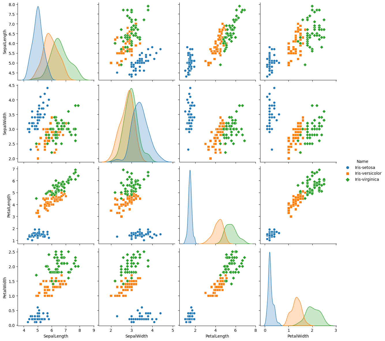
42.42.12.1. pairplot#
Pairwise is useful when you want to visualize the distribution of a variable or the relationship between multiple variables separately within subsets of your dataset.
import seaborn as sns

plt.figure()
sns.pairplot(iris, hue="Name", size=3, markers=["o", "s", "D"])
plt.show()
d:\Anaconda3\Lib\site-packages\seaborn\axisgrid.py:2095: UserWarning: The `size` parameter has been renamed to `height`; please update your code.
  warnings.warn(msg, UserWarning)
d:\Anaconda3\Lib\site-packages\seaborn\_oldcore.py:1119: FutureWarning: use_inf_as_na option is deprecated and will be removed in a future version. Convert inf values to NaN before operating instead.
  with pd.option_context('mode.use_inf_as_na', True):
d:\Anaconda3\Lib\site-packages\seaborn\_oldcore.py:1119: FutureWarning: use_inf_as_na option is deprecated and will be removed in a future version. Convert inf values to NaN before operating instead.
  with pd.option_context('mode.use_inf_as_na', True):
d:\Anaconda3\Lib\site-packages\seaborn\_oldcore.py:1119: FutureWarning: use_inf_as_na option is deprecated and will be removed in a future version. Convert inf values to NaN before operating instead.
  with pd.option_context('mode.use_inf_as_na', True):
d:\Anaconda3\Lib\site-packages\seaborn\_oldcore.py:1119: FutureWarning: use_inf_as_na option is deprecated and will be removed in a future version. Convert inf values to NaN before operating instead.
  with pd.option_context('mode.use_inf_as_na', True):
<Figure size 640x480 with 0 Axes>
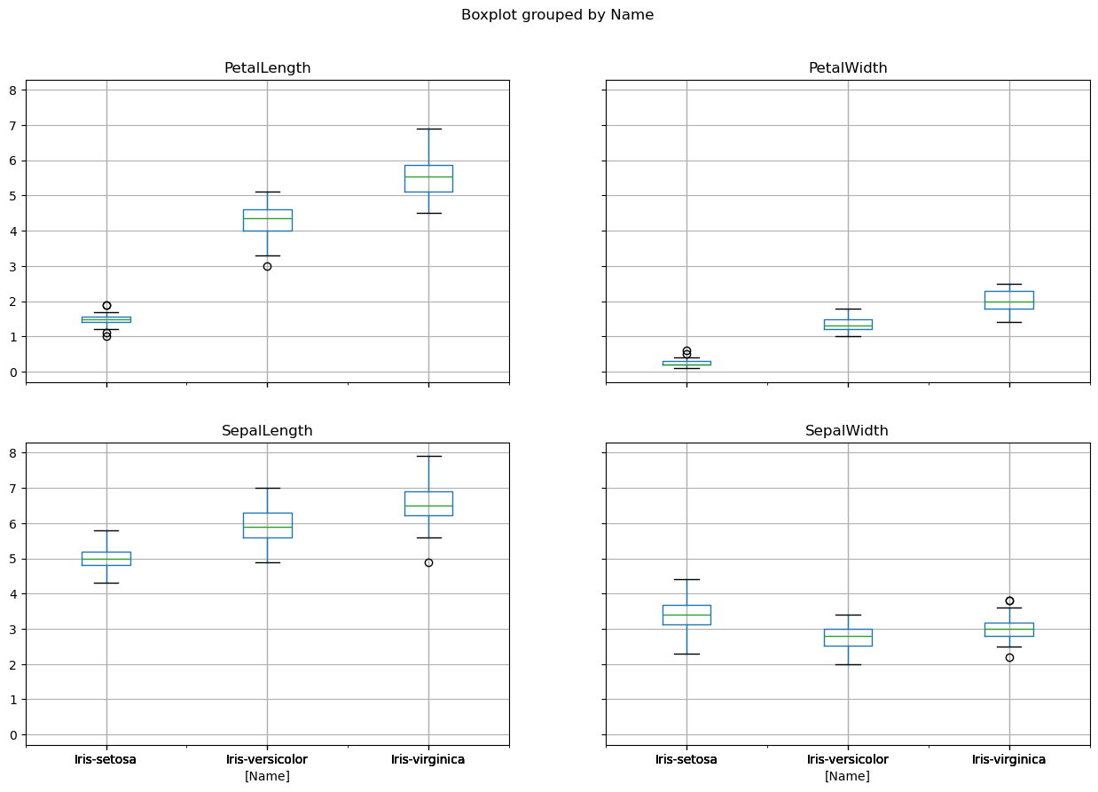
42.42.12.2. Boxplots#
plt.figure()
iris.boxplot(by="Name", figsize=(15, 10))
plt.show()
<Figure size 640x480 with 0 Axes>
42.42.12.3. 3D visualization#
You can also try to visualize high-dimensional datasets in 3D using color, shape, size and other properties of 3D and 2D objects. In this plot we use marks sizes to visualize fourth dimenssion which is Petal Width.
from mpl_toolkits.mplot3d import Axes3D
import matplotlib.pyplot as plt

# Assuming X and y are defined somewhere in your code

fig = plt.figure(1, figsize=(20, 15))
ax = Axes3D(fig, elev=48, azim=134)
ax.scatter(
    X[:, 0], X[:, 1], X[:, 2], c=y, cmap=plt.cm.Set1, edgecolor="k", s=X[:, 3] * 50
)

for name, label in [("Virginica", 0), ("Setosa", 1), ("Versicolour", 2)]:
    ax.text3D(
        X[y == label, 0].mean(),
        X[y == label, 1].mean(),
        X[y == label, 2].mean(),
        name,
        horizontalalignment="center",
        bbox=dict(alpha=0.5, edgecolor="w", facecolor="w"),
        size=25,
    )

ax.set_title("3D visualization", fontsize=40)
ax.set_xlabel("Sepal Length", fontsize=25)
ax.xaxis.set_ticklabels([])
ax.set_ylabel("Sepal Width", fontsize=25)
ax.yaxis.set_ticklabels([])
ax.set_zlabel("Petal Length", fontsize=25)
ax.zaxis.set_ticklabels([])

plt.show()
<Figure size 2000x1500 with 0 Axes>
42.42.13. Using KNN for classification#
42.42.13.1. Train the model#
# Fitting clasifier to the Training set
# Loading libraries
from sklearn.neighbors import KNeighborsClassifier

# Instantiate learning model (k = 3)
classifier = KNeighborsClassifier(n_neighbors=3)

# Fitting the model
classifier.fit(X_train, y_train)
KNeighborsClassifier(n_neighbors=3)In a Jupyter environment, please rerun this cell to show the HTML representation or trust the notebook.
On GitHub, the HTML representation is unable to render, please try loading this page with nbviewer.org.
KNeighborsClassifier(n_neighbors=3)
42.42.13.2. Predict, with test dataset#
y_pred = classifier.predict(X_test)
y_test
array([2, 1, 0, 2, 0, 2, 0, 1, 1, 1, 2, 1, 1, 1, 1, 0, 1, 1, 0, 0, 2, 1,
       0, 0, 2, 0, 0, 1, 1, 0])
y_pred
array([2, 1, 0, 2, 0, 2, 0, 1, 1, 1, 2, 1, 1, 1, 2, 0, 1, 1, 0, 0, 2, 1,
       0, 0, 2, 0, 0, 1, 1, 0])
42.42.13.3. Evaluating predictions#
# Building confusion matrix:
from sklearn.metrics import confusion_matrix

cm = confusion_matrix(y_test, y_pred)
print(cm)
[[11  0  0]
 [ 0 12  1]
 [ 0  0  6]]
from sklearn.metrics import accuracy_score

# Calculating model accuracy:
accuracy = accuracy_score(y_test, y_pred) * 100
print("Accuracy of our model is equal " + str(round(accuracy, 2)) + " %.")
Accuracy of our model is equal 96.67 %.
42.42.13.4. Using cross-validation for parameter tuning#
from sklearn.model_selection import cross_val_score

# creating list of K for KNN
k_list = list(range(1, 50, 2))
# creating list of cv scores
cv_scores = []

# perform 10-fold cross validation
for k in k_list:
    knn = KNeighborsClassifier(n_neighbors=k)
    scores = cross_val_score(knn, X_train, y_train, cv=10, scoring="accuracy")
    cv_scores.append(scores.mean())
# changing to misclassification error
MSE = [1 - x for x in cv_scores]

plt.figure()
plt.figure(figsize=(15, 10))
plt.title("The optimal number of neighbors", fontsize=20, fontweight="bold")
plt.xlabel("Number of Neighbors K", fontsize=15)
plt.ylabel("Misclassification Error", fontsize=15)
sns.set_style("whitegrid")
plt.plot(k_list, MSE)

plt.show()
<Figure size 640x480 with 0 Axes>
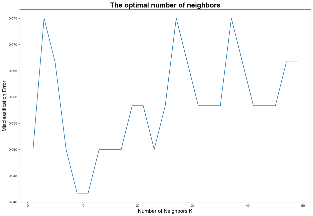
# finding best k
best_k = k_list[MSE.index(min(MSE))]
print("The optimal number of neighbors is %d." % best_k)
The optimal number of neighbors is 9.
42.42.14. Acknowledgments#
Thanks to SkalskiP for creating the open-source Kaggle jupyter notebook, licensed under Apache 2.0. It inspires the majority of the content of this assignment.