42.82. Boosting with tuning#

42.82.1. Introduction#

In this assginment, we will take you through the step by step approach in solving a House Pricing regression problem. This notebook aims to:

Provide insights on Housing Data
Understand importance of Preprocessing
Introduction to feature engineering
Use of ensembling algorithm

We hope that after reading this notebook, beginners will be more comfortable in tackling any learning problems and able to use the taught techniques to solve any problems from start to end. For non-beginners, hopefully you are able to get something out of it from this assignment and gain new insights and knowledge along the way.

42.82.2. Understanding data#

42.82.2.1. Task 1: Imports and load data#

import numpy as np # linear algebra
import pandas as pd # data processing, CSV file I/O (e.g. pd.read_csv)
import seaborn as sns
import matplotlib.pyplot as plt
sns.set_style("darkgrid")
from statsmodels.stats.outliers_influence import variance_inflation_factor
from sklearn.impute import SimpleImputer
import warnings

warnings.filterwarnings("ignore")

train = pd.read_csv('../../../assets/data/house_price_train.csv', index_col=0)
test = pd.read_csv('../../../assets/data/house_price_test.csv', index_col=0)


print("train: ", train.shape)
print("test: ", test.shape)
train.head()

Just taking a quick glance at the top rows of the dataframe, we can see that there are some columns that are filled with NAN (Not a Number). We will investigate this later on.

42.82.2.2. Task 2: Concatenate the train and test together#

What we did here is first to concatenate the train and test together for extracting insights into the Housing Price data as a whole. It will also be more convenient for our preprocessing steps later on as we will only have 1 data reference

X = pd.concat([train.drop("SalePrice", axis=1),test], axis=0)
y = train[['SalePrice']]

X.info()

42.82.2.3. Task 3: Isolate numerical and categorical columns#

Lets isolate both the numerical and categorical columns since we will be applying different visualization techniques on them

numeric_ = X.select_dtypes(exclude=['object']).drop(['MSSubClass'], axis=1).copy()
numeric_.columns

disc_num_var = ['OverallQual','OverallCond','BsmtFullBath','BsmtHalfBath','FullBath','HalfBath',
                'BedroomAbvGr', 'KitchenAbvGr', 'TotRmsAbvGrd', 'Fireplaces', 'GarageCars', 'MoSold', 'YrSold']

cont_num_var = []
for i in numeric_.columns:
    if i not in disc_num_var:
        cont_num_var.append(i)

cat_train = X.select_dtypes(include=['object']).copy()
cat_train['MSSubClass'] = X['MSSubClass']   #MSSubClass is nominal
cat_train.columns

42.82.2.4. Univariate Analysis#

42.82.2.4.1. Task 1: Numeric features#

For numerical features, we are always concerned about the distribution of these features, including the statistical characteristics of these columns e.g mean, median, mode. Hence we will usually use Distribution plot to visualize their data distribution. Boxplots are also commonly used to unearth the statistical characteristics of each feature. More often than not, we use it to look for any outliers that we might need to filter out later on during the preprocessing step.

fig = plt.figure(figsize=(18,16))
for index,col in enumerate(cont_num_var):
    plt.subplot(6,4,index+1)
    sns.distplot(numeric_.loc[:,col].dropna(), kde=False)
fig.tight_layout(pad=1.0)

Some of the Variables with mostly 1 value as seen from the plots above:

BsmtFinSF2
LowQualFinSF
EnclosedPorch
3SsnPorch
ScreenPorch
PoolArea
MiscVal

All these features are highly skewed, with mostly 0s. Having alot of 0s in the distribution doesnt really add information for predicting Housing Price. Hence, we will remove them during our preprocessing step

fig = plt.figure(figsize=(14,15))
for index,col in enumerate(cont_num_var):
    plt.subplot(6,4,index+1)
    sns.boxplot(y=col, data=numeric_.dropna())
fig.tight_layout(pad=1.0)

fig = plt.figure(figsize=(20,15))
for index,col in enumerate(disc_num_var):
    plt.subplot(5,3,index+1)
    sns.countplot(x=col, data=numeric_.dropna())
fig.tight_layout(pad=1.0)

42.82.2.4.2. Task 2: Categorical features#

In the case of categorical features, we will often use countplots to visualize the count of each distinct value within each features. We can see that some categorical features like Utilities, Condition2 consist of mainly just one value, which does not add any useful information. Thus, we will also remove them later on.

fig = plt.figure(figsize=(18,20))
for index in range(len(cat_train.columns)):
    plt.subplot(9,5,index+1)
    sns.countplot(x=cat_train.iloc[:,index], data=cat_train.dropna())
    plt.xticks(rotation=90)
fig.tight_layout(pad=1.0)

Univariate Analysis helps us to understand all the features better, on an individual scale. To further deepen our insights and uncover potential pattern in the data, we will also need to find out more about the relationship between all these features with one another, which brings us to our next step in our analysis - Bivariate Analysis

42.82.2.5. Bi-Variate Analysis#

Bi-variate analysis looks at 2 different features to identify any possible relationship or distinctive patterns between the 2 features. One of the commonly used technique is through the Correlation Matrix. Correlation matrix is an effective tool to uncover linear relationship (Correlation) between any 2 continuous features. Correlation not only allow us to determine which features are important to Saleprice, but also as a mean to investigate any multicollinearity between our independent predictors.
Multicollinearity happens when 2 or more independent variables are highly correlated with one another. In such situation, it causes precision loss in our regression coefficients, affecting our ability to identify the most important features that are most useful to our model

42.82.2.5.1. Task 1: Correlation matrix#

plt.figure(figsize=(14,12))
correlation = numeric_.corr()
sns.heatmap(correlation, mask = correlation <0.8, linewidth=0.5, cmap='Blues')

Highly Correlated variables:

GarageYrBlt and YearBuilt
TotRmsAbvGrd and GrLivArea
1stFlrSF and TotalBsmtSF
GarageArea and GarageCars

From the correlation matrix we have identified the above variables which are highly correlated with each other. This finding will guide us in our preprocessing steps later on as we aim to remove highly correlated features to avoid performance loss in our model

42.82.2.5.2. Task 2: Identifying relationship between Numerical Predictor and Target (SalePrice)#

Below, we sorted the strength of linear relationship between Saleprice and other features. OverallQual and GrLivArea has the strongest linear relationship with SalePrice. Hence, these 2 features will be important factor in predicting Housing Price

numeric_train = train.select_dtypes(exclude=['object'])
correlation = numeric_train.corr()
correlation[['SalePrice']].sort_values(['SalePrice'], ascending=False)

42.82.2.5.3. Task 3: Scatterplot#

Using scatterplot can also help us to identify potential linear relationship between Numerical features. Although scatterplot does not provide quantitative evidence on the strength of linear relationship between our features, it is useful in helping us to visualize any sort of relationship that correlation matrix could not calculate. E.g Quadratic, Exponential relationships.

fig = plt.figure(figsize=(20,20))
for index in range(len(numeric_train.columns)):
    plt.subplot(10,5,index+1)
    sns.scatterplot(x=numeric_train.iloc[:,index], y='SalePrice', data=numeric_train.dropna())
fig.tight_layout(pad=1.0)

42.82.3. Data Processing#

Now that we have more or less finished analysing our data and gaining insights through the various analysis and visualization, we will have to leverage on these insights to guide our preprocessing decision, so as to provide a clean and error-free data for our model to train on later on.

We do not perform visualization and analysis just to create pretty graphs or for the sake of doing it, IT IS VITAL TO OUR PREPROCESSING!

This section outlines the steps for Data Processing:

Removing Redundant Features
Dealing with Outliers
Filling in missing values

42.82.3.1. Removing redundant features#

42.82.3.1.1. Task 1：Features with multicollinearity#

From the above correlation matrix, we have pinpointed certain features that are highly correlated

GarageYrBlt and YearBuilt
TotRmsAbvGrd and GrLivArea
1stFlrSF and TotalBsmtSF
GarageArea and GarageCars

We will remove the highly correlated features to avoid the problem of multicollinearity explained earlier

X.drop(['GarageYrBlt','TotRmsAbvGrd','1stFlrSF','GarageCars'], axis=1, inplace=True)

42.82.3.1.2. Task 2: Features with a lot of missing values#

Apart from these highly correlated features, we will also remove features that is not very useful in prediction due to many missing values. PoolQC, MiscFeature, Alley has too many missing values to provide any useful information

plt.figure(figsize=(25,8))
plt.title('Number of missing rows')
missing_count = pd.DataFrame(X.isnull().sum(), columns=['sum']).sort_values(by=['sum'],ascending=False).head(20).reset_index()
missing_count.columns = ['features','sum']
sns.barplot(x='features',y='sum', data = missing_count)

X.drop(['PoolQC','MiscFeature','Alley'], axis=1, inplace=True)

42.82.3.1.3. Task 3: Useless features in predicting SalePrice#

We will also remove features that does not have any linear relationship with target SalePrice. We can see from the plot below that the MoSold and YrSold does not have any impact on the price of the house sold.

fig,axes = plt.subplots(1,2, figsize=(15,5))
sns.regplot(x=numeric_train['MoSold'], y='SalePrice', data=numeric_train, ax = axes[0], line_kws={'color':'black'})
sns.regplot(x=numeric_train['YrSold'], y='SalePrice', data=numeric_train, ax = axes[1],line_kws={'color':'black'})
fig.tight_layout(pad=2.0)

correlation[['SalePrice']].sort_values(['SalePrice'], ascending=False).tail(10)

X.drop(['MoSold','YrSold'], axis=1, inplace=True)

42.82.3.1.4. Task 4: Removing features that have mostly just 1 value#

Earlier during our Univariate analysis, we found that some features mostly consist of just a single value or 0s, which is not useful to us. Therefore, we set a user defined threshold at 96%. If a column has more than 96% of the same value, we will render the features to be useless and remove it, since there isnt much information we can extract from

cat_col = X.select_dtypes(include=['object']).columns
overfit_cat = []
for i in cat_col:
    counts = X[i].value_counts()
    zeros = counts.iloc[0]
    if zeros / len(X) * 100 > 96:
        overfit_cat.append(i)

overfit_cat = list(overfit_cat)
X = X.drop(overfit_cat, axis=1)

num_col = X.select_dtypes(exclude=['object']).drop(['MSSubClass'], axis=1).columns
overfit_num = []
for i in num_col:
    counts = X[i].value_counts()
    zeros = counts.iloc[0]
    if zeros / len(X) * 100 > 96:
        overfit_num.append(i)

overfit_num = list(overfit_num)
X = X.drop(overfit_num, axis=1)

print("Categorical Features with >96% of the same value: ",overfit_cat)
print("Numerical Features with >96% of the same value: ",overfit_num)

42.82.3.2. Dealing with outliers#

Removing outliers will prevent our models performance from being affected by extreme values.
From our boxplot earlier, we have pinpointed the following features with extreme outliers:

LotFrontage
LotArea
BsmtFinSF1
TotalBsmtSF
GrLivArea

We will remove the outliers based on certain threshold value.

out_col = ['LotFrontage','LotArea','BsmtFinSF1','TotalBsmtSF','GrLivArea']
fig = plt.figure(figsize=(20,5))
for index,col in enumerate(out_col):
    plt.subplot(1,5,index+1)
    sns.boxplot(y=col, data=X)
fig.tight_layout(pad=1.5)

train = train.drop(train[train['LotFrontage'] > 200].index)
train = train.drop(train[train['LotArea'] > 100000].index)
train = train.drop(train[train['BsmtFinSF1'] > 4000].index)
train = train.drop(train[train['TotalBsmtSF'] > 5000].index)
train = train.drop(train[train['GrLivArea'] > 4000].index)

X.shape

42.82.3.3. Filling Missing Values#

Our machine learning model is unable to deal with missing values, thus we need to deal with them based on our understanding of the features. These missing values are denoted NAN as we have seen earlier during our data exploration.

pd.DataFrame(X.isnull().sum(), columns=['sum']).sort_values(by=['sum'],ascending=False).head(15)

42.82.3.3.1. Task 1: Ordinal features#

We will replace the ordinal missing values with NA, which will be mapped later on when we encode them into an ordered arrangement

cat = ['GarageType','GarageFinish','BsmtFinType2','BsmtExposure','BsmtFinType1', 
       'GarageCond','GarageQual','BsmtCond','BsmtQual','FireplaceQu','Fence',"KitchenQual",
       "HeatingQC",'ExterQual','ExterCond']

X[cat] = X[cat].fillna("NA")

42.82.3.3.2. Task 2: Categorical features#

We will replace the missing value of our categorical features with the most frequent occurrence (mode) of the individual features.

#categorical
cols = ["MasVnrType", "MSZoning", "Exterior1st", "Exterior2nd", "SaleType", "Electrical", "Functional"]
X[cols] = X.groupby("Neighborhood")[cols].transform(lambda x: x.fillna(x.mode()[0]))

42.82.3.3.3. Task 3: Numerical features#

For Numerical Features, the common approach will be to replace the missing value with the mean of the feature distribution.
However, certain features like LotFrontage and GarageArea have wide variance in their distribution. Taking mean values across Neighborhoods, we will see that the mean varies alot from just taking the mean value of these individual column, since each neightborhood have different LotFrontage and GarageArea mean value. Hence, i decided to group these features by Neighborhoods to impute the respective mean values.

Note: My initial approach was based on the means of both train and test set. This exposed us to the issue of data leakage, where information from the test set is used to compute mean values. The right way to do it will be to impute solely based on the mean of the train data.

print("Mean of LotFrontage: ", X['LotFrontage'].mean())
print("Mean of GarageArea: ", X['GarageArea'].mean())

neigh_lot = X.groupby('Neighborhood')['LotFrontage'].mean().reset_index(name='LotFrontage_mean')
neigh_garage = X.groupby('Neighborhood')['GarageArea'].mean().reset_index(name='GarageArea_mean')

fig, axes = plt.subplots(1,2,figsize=(22,8))
axes[0].tick_params(axis='x', rotation=90)
sns.barplot(x='Neighborhood', y='LotFrontage_mean', data=neigh_lot, ax=axes[0])
axes[1].tick_params(axis='x', rotation=90)
sns.barplot(x='Neighborhood', y='GarageArea_mean', data=neigh_garage, ax=axes[1])

#for correlated relationship
X['LotFrontage'] = X.groupby('Neighborhood')['LotFrontage'].transform(lambda x: x.fillna(x.mean()))
X['GarageArea'] = X.groupby('Neighborhood')['GarageArea'].transform(lambda x: x.fillna(x.mean()))
X['MSZoning'] = X.groupby('MSSubClass')['MSZoning'].transform(lambda x: x.fillna(x.mode()[0]))

#numerical
cont = ["BsmtHalfBath", "BsmtFullBath", "BsmtFinSF1", "BsmtFinSF2", "BsmtUnfSF", "TotalBsmtSF", "MasVnrArea"]
X[cont] = X[cont] = X[cont].fillna(X[cont].mean())

42.82.3.3.4. Task 4: Changing Data Type#

Since MSSubClass is an integer column based on some mapped values in string notation, we change its data type to string value instead

X['MSSubClass'] = X['MSSubClass'].apply(str)

42.82.3.3.5. Task 5: Mapping ordinal features#

There are some columns which are ordinal by nature, which represents the quality or condition of certain housing features. In this case, we will map the respective strings to a value. The better the quality, the higher the value

ordinal_map = {'Ex': 5,'Gd': 4, 'TA': 3, 'Fa': 2, 'Po': 1, 'NA':0}
fintype_map = {'GLQ': 6,'ALQ': 5,'BLQ': 4,'Rec': 3,'LwQ': 2,'Unf': 1, 'NA': 0}
expose_map = {'Gd': 4, 'Av': 3, 'Mn': 2, 'No': 1, 'NA': 0}
fence_map = {'GdPrv': 4,'MnPrv': 3,'GdWo': 2, 'MnWw': 1,'NA': 0}

ord_col = ['ExterQual','ExterCond','BsmtQual', 'BsmtCond','HeatingQC','KitchenQual','GarageQual','GarageCond', 'FireplaceQu']
for col in ord_col:
    X[col] = X[col].map(ordinal_map)
    
fin_col = ['BsmtFinType1','BsmtFinType2']
for col in fin_col:
    X[col] = X[col].map(fintype_map)

X['BsmtExposure'] = X['BsmtExposure'].map(expose_map)
X['Fence'] = X['Fence'].map(fence_map)

After removing the outliers, highly correlated features and imputing missing values, we can now proceed with adding additional information for our model to train on. This is done by the means of - Feature Engineering.

42.82.4. Feature engineering#

Feature Engineering is a technique by which we create new features that could potentially aid in predicting our target variable, which in this case, is SalePrice. In this notebook, we will create additional features based on our Domain Knowledge of the housing features

Based on the current feature we have, the first additional featuire we can add would be TotalLot, which sums up both the LotFrontage and LotArea to identify the total area of land available as lot. We can also calculate the total number of surface area of the house, TotalSF by adding the area from basement and 2nd floor. TotalBath can also be used to tell us in total how many bathrooms are there in the house. We can also add all the different types of porches around the house and generalise into a total porch area, TotalPorch.

TotalLot = LotFrontage + LotArea
TotalSF = TotalBsmtSF + 2ndFlrSF
TotalBath = FullBath + HalfBath
TotalPorch = OpenPorchSF + EnclosedPorch + ScreenPorch
TotalBsmtFin = BsmtFinSF1 + BsmtFinSF2

X['TotalLot'] = X['LotFrontage'] + X['LotArea']
X['TotalBsmtFin'] = X['BsmtFinSF1'] + X['BsmtFinSF2']
X['TotalSF'] = X['TotalBsmtSF'] + X['2ndFlrSF']
X['TotalBath'] = X['FullBath'] + X['HalfBath']
X['TotalPorch'] = X['OpenPorchSF'] + X['EnclosedPorch'] + X['ScreenPorch']

42.82.4.1. Task 1: Binay columns#

We also include simple feature engineering by creating binary columns for some features that can indicate the presence(1) / absence(0) of some features of the house

colum = ['MasVnrArea','TotalBsmtFin','TotalBsmtSF','2ndFlrSF','WoodDeckSF','TotalPorch']

for col in colum:
    col_name = col+'_bin'
    X[col_name] = X[col].apply(lambda x: 1 if x > 0 else 0)

42.82.4.2. Task 2: Converting categorical to numerical#

Lastly, because machine learning only learns from data that is numerical in nature, we will convert the remaining categorical columns into one-hot features using the get_dummies() method into numerical columns that is suitable for feeding into our machine learning algorithm.

X = pd.get_dummies(X)

42.82.4.3. Task 3: SalePrice distribution#

plt.figure(figsize=(10,6))
plt.title("Before transformation of SalePrice")
dist = sns.distplot(train['SalePrice'],norm_hist=False)

Distribution is skewed to the right, where the tail on the curve’s right-hand side is longer than the tail on the left-hand side, and the mean is greater than the mode. This situation is also called positive skewness.
Having a skewed target will affect the overall performance of our machine learning model, thus, one way to alleviate will be to using log transformation on skewed target, in our case, the SalePrice to reduce the skewness of the distribution.

plt.figure(figsize=(10,6))
plt.title("After transformation of SalePrice")
dist = sns.distplot(np.log(train['SalePrice']),norm_hist=False)

y["SalePrice"] = np.log(y['SalePrice'])

Now that we are satisfied with our final data, we will proceed to the part where we will solve this regression problem - Modeling

42.82.5. Modeling#

This section will consist of scaling the data for better optimization in our training, and also introducing the varieties of ensembling methods that are used in this notebook for predicting the Housing price. We also try out hyperparameter tuning briefly, as i will be dedicating a new notebook that will explain more in details on the process of Hyperparameter Tuning as well as the mathematical aspect of the ensemble algorithms.

42.82.5.1. Split into train-validation set#

x = X.loc[train.index]
y = y.loc[train.index]
test = X.loc[test.index]

42.82.5.2. Scaling of Data#

RobustScaler is a transformation technique that removes the median and scales the data according to the quantile range (defaults to IQR: Interquartile Range). The IQR is the range between the 1st quartile (25th quantile) and the 3rd quartile (75th quantile). It is also robust to outliers, which makes it ideal for data where there are too many outliers that will drastically reduce the number of training data.

Previously i fitted the RobustScaler on both Train and Test set, and that is a mistake on my side. By fitting the scaler on both train and testset, we exposed ourselves to the problem of Data Leakage. Data Leakage is a problem when information from outside the training dataset is used to create the model. If we fit the scaler on both training and test data, our training data characteristics will contain the distribution of our testset. As such, we are unknowningly passing in information about our test data into the final training data for training, which will not give us the opportunity to truly test our model on data it has never seen before.
Lesson Learnt: Fit the scaler just on training data, and then transforming it on both training and test data

from sklearn.preprocessing import RobustScaler

cols = x.select_dtypes(np.number).columns
transformer = RobustScaler().fit(x[cols])
x[cols] = transformer.transform(x[cols])
test[cols] = transformer.transform(test[cols])

42.82.5.3. Ensemble Algorithms#

from sklearn.model_selection import train_test_split

X_train, X_val, y_train, y_val = train_test_split(x, y, test_size=0.2, random_state=2020)

42.82.5.3.1. Task 1: Ensembling models#

Ensembling methods are meta-algorithms which involves combining several machine learning models into one predictive model, aim at decreasing variance(reduce overfitting) and improving bias(improve accuracy).
The 3 main ensembling methods are Bagging, Boosting and Stacking.
In this notebook, we will focus mainly on Boosting, which is what we will be using for our prediction.

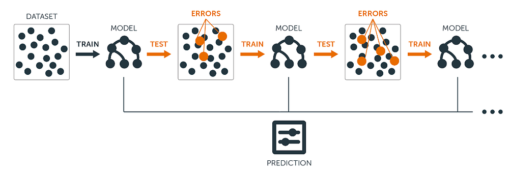
Boosting works on a class of weak learners, improving them into strong learners. It is being improved sequentially where the misclassified instances will be given more weights so that during the subsequent training, the learner will place more emphasis in correcting the previously misclassfied instance, less so on the already correctly identified instances. Over time, the eventual learner will possess the ability to predict accurately as a result of learning from past mistakes

from sklearn.metrics import mean_squared_error, mean_absolute_error
from xgboost import XGBRegressor
from sklearn import ensemble
from lightgbm import LGBMRegressor
from sklearn.model_selection import cross_val_score
from catboost import CatBoostRegressor

42.82.5.3.2. Task 2: XGBoost#

Extreme Gradient Boost (XGB) is a boosting algorithm that uses the gradient boosting framework; where gradient descent algorithm is employed to minimize the errors in the sequential model. It improves on the gradient boosting framework with faster execution speed and improved performance.

xgb = XGBRegressor(booster='gbtree', objective='reg:squarederror', tree_method='gpu_hist')

XGBoost hyperParameter tuning

from sklearn.model_selection import RandomizedSearchCV

param_lst = {
    'learning_rate' : [0.01, 0.1, 0.15, 0.3, 0.5],
    'n_estimators' : [100, 500, 1000, 2000, 3000],
    'max_depth' : [3, 6, 9],
    'min_child_weight' : [1, 5, 10, 20],
    'reg_alpha' : [0.001, 0.01, 0.1],
    'reg_lambda' : [0.001, 0.01, 0.1]
}

xgb_reg = RandomizedSearchCV(estimator = xgb, param_distributions = param_lst,
                              n_iter = 100, scoring = 'neg_root_mean_squared_error',
                              cv = 5)
       
xgb_search = xgb_reg.fit(X_train, y_train)

# XGB with tune hyperparameters
best_param = xgb_search.best_params_
xgb = XGBRegressor(tree_method='gpu_hist', **best_param)

42.82.5.3.3. Task 3: LightGBM#

LightBGM is another gradient boosting framework developed by Microsoft that is based on decision tree algorithm, designed to be efficient and distributed. Some of the advantages of implementing LightBGM compared to other boosting frameworks include:

Faster training speed and higher efficiency (use histogram based algorithm i.e it buckets continuous feature values into discrete bins which fasten the training procedure)
Lower memory usage (Replaces continuous values to discrete bins which result in lower memory usage)
Better accuracy
Support of parallel and GPU learning
Capable of handling large-scale data (capable of performing equally good with large datasets with a significant reduction in training time as compared to XGBOOST)

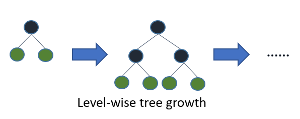
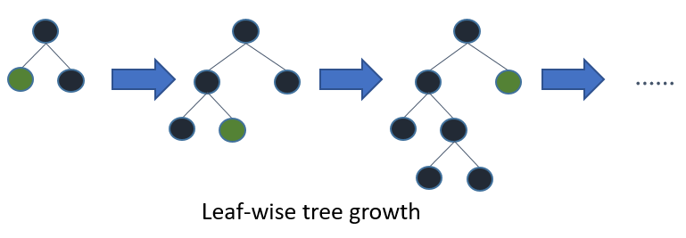
LightGBM splits the tree leaf wise with the best fit whereas other boosting algorithms split the tree depth wise or level wise rather than leaf-wise. This leaf-wise algorithm reduces more loss than the level-wise algorithm, hence resulting in much better accuracy which can rarely be achieved by any of the existing boosting algorithms.

lgbm = LGBMRegressor(boosting_type='gbdt',objective='regression', max_depth=-1,
                    lambda_l1=0.0001, lambda_l2=0, learning_rate=0.1,
                    n_estimators=100, max_bin=200, min_child_samples=20, 
                    bagging_fraction=0.75, bagging_freq=5,
                    bagging_seed=7, feature_fraction=0.8,
                    feature_fraction_seed=7, verbose=-1, device='gpu')

LightBGM Hyperparameter tuning

param_lst = {
    'max_depth' : [2, 5, 8, 10],
    'learning_rate' : [0.001, 0.01, 0.1, 0.2],
    'n_estimators' : [100, 300, 500, 1000, 1500],
    'lambda_l1' : [0.0001, 0.001, 0.01],
    'lambda_l2' : [0, 0.0001, 0.001, 0.01],
    'feature_fraction' : [0.4, 0.6, 0.8],
    'min_child_samples' : [5, 10, 20, 25]
}

lightgbm = RandomizedSearchCV(estimator = lgbm, param_distributions = param_lst,
                              n_iter = 100, scoring = 'neg_root_mean_squared_error',
                              cv = 5)
       
lightgbm_search = lightgbm.fit(X_train, y_train)

# LightBGM with tuned hyperparameters
best_param = lightgbm_search.best_params_
lgbm = LGBMRegressor(**best_param)

42.82.5.3.4. Task 4: Catboost#

Catboost is another alternative gradient boosting framework developed by Yandex. The word “Catboost” is derived from two words; “Category” and “Boosting”. This means that Catboost itself can deal with categorical features which usually has to be converted to numerical encodings in order to feed into traditional gradient boost frameworks and machine learning models.
The 2 critical features in Catboost algorithm is the use of ordered boosting and innovative algorithm for processing categorical features, which fight the prediction shift caused by a special kind of target leakage present in all existing implementations of gradient boosting algorithms.
Find out more here

cb = CatBoostRegressor(loss_function='RMSE', logging_level='Silent', task_type='GPU')

CatBoost Hyperparameter Tuning

param_lst = {
    'n_estimators' : [100, 300, 500, 1000, 1300, 1600],
    'learning_rate' : [0.0001, 0.001, 0.01, 0.1],
    'l2_leaf_reg' : [0.001, 0.01, 0.1],
    'random_strength' : [0.25, 0.5 ,1],
    'max_depth' : [3, 6, 9],
    'min_child_samples' : [2, 5, 10, 15, 20],
    
}

catboost = RandomizedSearchCV(estimator = cb, param_distributions = param_lst,
                              n_iter = 100, scoring = 'neg_root_mean_squared_error',
                              cv = 5)

catboost_search = catboost.fit(X_train, y_train)

# CatBoost with tuned hyperparams
best_param = catboost_search.best_params_
cb = CatBoostRegressor(logging_level='Silent', task_type='GPU', **best_param)

42.82.5.3.5. Task 5: Training and evaluation#

def mean_cross_val(model, X, y):
    score = cross_val_score(model, X, y, cv=5)
    mean = score.mean()
    return mean

cb.fit(X_train, y_train)   
preds = cb.predict(X_val) 
preds_test_cb = cb.predict(test)
mae_cb = mean_absolute_error(y_val, preds)
rmse_cb = np.sqrt(mean_squared_error(y_val, preds))
score_cb = cb.score(X_val, y_val)
cv_cb = mean_cross_val(cb, x, y)


xgb.fit(X_train, y_train)   
preds = xgb.predict(X_val) 
preds_test_xgb = xgb.predict(test)
mae_xgb = mean_absolute_error(y_val, preds)
rmse_xgb = np.sqrt(mean_squared_error(y_val, preds))
score_xgb = xgb.score(X_val, y_val)
cv_xgb = mean_cross_val(xgb, x, y)


lgbm.fit(X_train, y_train)   
preds = lgbm.predict(X_val) 
preds_test_lgbm = lgbm.predict(test)
mae_lgbm = mean_absolute_error(y_val, preds)
rmse_lgbm = np.sqrt(mean_squared_error(y_val, preds))
score_lgbm = lgbm.score(X_val, y_val)
cv_lgbm = mean_cross_val(lgbm, x, y)

model_performances = pd.DataFrame({
    "Model" : ["XGBoost", "LGBM", "CatBoost"],
    "CV(5)" : [str(cv_xgb)[0:5], str(cv_lgbm)[0:5], str(cv_cb)[0:5]],
    "MAE" : [str(mae_xgb)[0:5], str(mae_lgbm)[0:5], str(mae_cb)[0:5]],
    "RMSE" : [str(rmse_xgb)[0:5], str(rmse_lgbm)[0:5], str(rmse_cb)[0:5]],
    "Score" : [str(score_xgb)[0:5], str(score_lgbm)[0:5], str(score_cb)[0:5]]
})

print("Sorted by Score:")
print(model_performances.sort_values(by="Score", ascending=False))

42.82.5.3.6. Task 6 Blending#

Blending is a technique that give different weightage to different algorithms that will affect their influence of the predictions. Such techniques can help to improve performance since it uses a variety of models as predictors. Special thanks to @itslek for the implementation of blending. I have randomly chosen the weights for each models in this case, however, you can improve on this by futher tuning the weightage to be given to each model to achieve a better accuracy!

def blend_models_predict(X, b, c, d):
       return ((b* xgb.predict(X)) + (c * lgbm.predict(X)) + (d * cb.predict(X)))

subm = np.exp(blend_models_predict(test, 0.4, 0.3, 0.3))
submission = pd.DataFrame({'Id': test.index,
                           'SalePrice': subm})

Hope you guys have learnt how the whole process of solving a regression problems looks like, understood the importance of data preprocessing and gain insights into the varieties of ensembling algorithms that you can use in future regression problems.

42.82.6. Acknowledgments#

Thanks to aqx for creating the open-source course Data Science Workflow TOP 2% (with Tuning). It inspires the majority of the content in this chapter.

Ocademy Open Machine Learning Book

Boosting with tuning

Contents